How to Create Your First PivotTable in Microsoft Excel

We all deal with data overload. More than ever, we need easy ways to take a large dataset and find meaning inside of it. If you work with spreadsheets in Microsoft Excel, PivotTables are an ideal solution for data overload. Few tools are as easy to use and powerful as PivotTables.

With a PivotTable, you can point Excel to a list of data and easily summarize it in a few clicks. You can quickly segment your data, calculating and summarizing it by dragging and dropping fields.

In this tutorial, I'll teach you how to create a PivotTable in Excel. At the end of this tutorial, you'll have the skills to summarize data in spreadsheets using one of Excel's most powerful features.

What's a PivotTable?

A PivotTable is a tool to make sense of a huge list of data. When you have a large spreadsheet with many rows, it's helpful to summarize your data in an Excel PivotTable.

Here's a simple example: you have a big list of clients you billed as part of your freelance work. Each row is a project or product we've billed a client for. At the end of the year, how can I review my work and see how I spent my time?

From a spreadsheet, it can be overwhelming to understand your data. What if I wanted to know the total amount I billed each client? Sure, I could filter by each client and sum it up, but there's a much easier way to do it.

A PivotTable helps us summarize and understand data. In the example below, I created an Excel PivotTable out of the spreadsheet, and summed up my billings per client. 

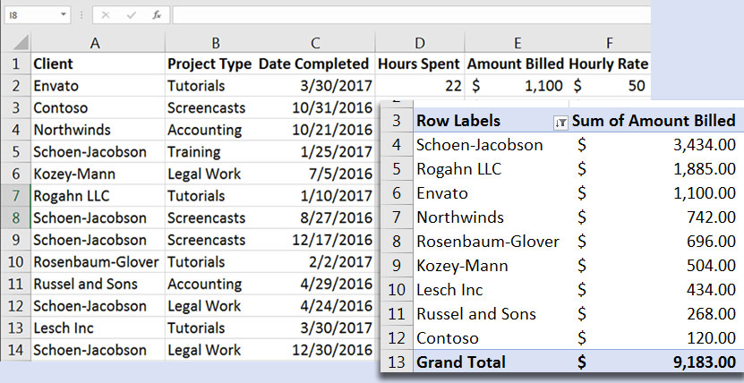
The PivotTable, shown on the right, is a great way to summarize the data. I've shown each "Client" as its own row, and summed up my "amount billed." 

Notice that in the original spreadsheet, I've done several different rounds of work for a client named "Schoen-Jacobson." The PivotTable sums up my billings to them on a single line, which is very convenient.

You can drag and drop fields to slice the data and view it in a variety of ways. In the examples below, I've used the same PivotTable with different row types to understand my data better.

In short, PivotTables are a tool to tame and understand the data in your spreadsheets with better. Learning how to create PivotTables in Excel will help you make sense of your data. Let's get started.

How to Create an Excel PivotTable (Watch & Learn)

Sometimes, you have to see a tool like PivotTables in action to think about how you can use it. Check out the video below to learn how to create a PivotTable in Excel quickly:

If you want a step-by-step guide on creating your first PivotTable in Excel, keep reading the tutorial to find out more. I'll walk you through how to create a PivotTable and understand your data better.

1. Prepare Your Excel PivotTable

If you want to follow along with this tutorial, download the example workbook that's included with this tutorial. I've filled in some data in a workbook so that you can create a PivotTable in Excel and follow along with this tutorial.

If you're using your own data, no problem. Before we create a a PivotTable, we need to make sure that our data will work well in a PivotTable. Here are my keys to preparing data for a PivotTable:

1. Each row of the data should be a record of its own. Basically, you can use each line for your data.


2. Make sure that each column has a header, and ensure there are no blank columns in your data.

2. Create the PivotTable in Excel

We're ready to create our first PivotTable. Start by highlighting the columns that contain your data, and then find the Insert tab on the Excel ribbon.

With your data highlighted, click on the PivotTable button on the far left of the Insert tab to create your first PivotTable.

Now, a new window will pop up to finish creating the PivotTable in Excel. I typically leave these settings at their default, which will create a PivotTable on a sheet of its own. Go ahead and press OK, and Excel will create the PivotTable.

3. Drag and Drop Your Fields

Once you've created the PivotTable, Excel will take you to the new sheet to build your PivotTable. I think of this screen as a drag-and-drop report builder. Here's how to read this menu:

On the right side of the screen is a menu labeled PivotTable Fields. You'll see each of the columns from your data in the list, which are called fields in a PivotTable.

At the bottom of the menu are four boxes: Filters, Columns, Rows, and Values. You can drag and drop any field into any of the boxes. 

Let's start off by dragging Client down into the Rows box. Click and drag Client from the fields list, and drag it down into the white box below Rows.

Now we're getting somewhere! Because we placed the Clients field in the Rows box, the PivotTable put each client on its own row. 

This is how PivotTables work: you can drag and drop the fields into the various boxes, and the PivotTable will show that field in the box you drag it to. You can show a field as a Filter, Row, Column, or Value.

In the screenshot below, here's another quick example. I dragged and dropped the Project Type to the Columns field. Now, our Excel PivotTable shows each of the project types in our original data as a column of its own.

I'll go ahead and undo these changes, and move Client back to the Rows box.

What if we wanted to know how much we billed each client? Remember that we have that in our original data, in the Amount Billed column. We need to add the amounts to the table as well.

Since we want to see those amounts as numeric values, let's drag Amount Billed to the Values box (lower right corner).

Now, we have a listing of the number of times that we've billed each client for work. The second column counts up each time we've worked with a client, and shows the count total.

However, we don't want to see the count of the projects we did for each client. We want to know the total dollars, or the sum of what we billed them instead.

Let's right click on the numbers in the second column. Find the option that reads Summarize Values By and choose Sum. You'll see now that the amounts are being summed up, and we can see the total dollars for each client.

We've built our first useful PivotTable, summing up our billings by client.  Now, let's add a second field to see even more detail.

What if we wanted to segment our data even further? Let's say that we wanted to see not only the client, but also the type of work that we did for that client. 

To do that, let's take the Project Type field and drag it down into the Rows box, and drag it above Client. 

Now, our PivotTable has two levels of detail: it sums our work up by project type (Accounting, Legal Work, Screencasts, Training, and Tutorials), and then shows the client for each type of work. We've added two levels of detail to the Excel PivotTable so that we can see top clients for each type of work.

By now, you should have some ideas of how you might be able to use PivotTables to assist your freelance work or small business. If you have spreadsheets with data and need to understand them, try throwing it into a PivotTable and re-arranging fields to understand the data more.

Recap and Keep Learning

PivotTables are one of the most powerful tools I know of in Excel. If you want to keep learning Excel skills, check out the tutorials below:

• Bob Flisser has an Advanced PivotTable tutorial that teaches you to Combine Data from Multiple Sheets into a single PivotTable.


• If you need to clean up your spreadsheet before creating a PivotTable, here's How to Find and Remove Duplicates.


• If you'd like a more basic introduction to Excel functions, check out our series How to Make and Use Excel Formulas.
  

Do you have any questions about how to use a PivotTable? If so, let me know in the comments below.