How To Make Use of 5 Advanced Excel Pivot Table Techniques

The problem we all face isn't a lack of data; instead, it's finding meaning in huge amounts of data! That's why I advocate for the use of PivotTables, an amazing feature in Excel to summarize and analyze your data.

As a finance professional, I'm genetically inclined to love spreadsheets. But I also find that I use spreadsheets to organize my creative and freelance work. No matter what you use spreadsheets for, a PivotTable can help you find greater meaning in the data.

In this tutorial, we'll build upon on our starter tutorials on using PivotTables to work better with your data. I'll show you five of my favorite advanced PivotTable techniques. 

Throughout this tutorial, I'll use sample data provided by Microsoft on this page. Use this data to recreate the examples or test the features I'm showcasing.

How to Use Advanced Pivot Table Techniques in Excel (Quick Video)

I love teaching with screencasts, which give you a chance to watch me use the features step-by-step. Check out the quick video below which cover five of my favorite advanced Excel PivotTable features:

5 Advanced Excel Pivot Table Techniques

Keep reading for a walkthrough of how to use each of these five features in the written tutorial below, covering: Slicers, Timelines, Tabular View, Calculated Fields, and Recommended PivotTables. Let's get into it.

1. Slicers

Slicers are point and click tools to refine the data included in your Excel PivotTable. Insert a slicer, and you can easily change the data that's included in your PivotTable.

Many times, I'm developing PivotTable reports that will be used by many others. Adding slicers can help my end user customize the report to their liking.

To add a slicer, click within your PivotTable and find the Analyze tab on Excel's ribbon.

Hold Control on your keyboard to multi-select items within a slicer, which will include multiple selections from a column as part of your PivotTable data.

2. Timelines

Timelines are a special type of slicer, used to tweak the dates included as part of your PivotTable data. If your data includes dates in it, you really need to try out Timelines as a way to select data from specific time periods.

Tip: If this feature isn't working for you, make sure that your original data has the date formatted as a date in the spreadsheet.

To add a Timeline, make sure that you've selected a PivotTable (click within it) and then click on the Insert > Timeline option on Excel's ribbon. On the pop-up window, check the box of your date column (or multiple columns) and press OK to create a timeline.

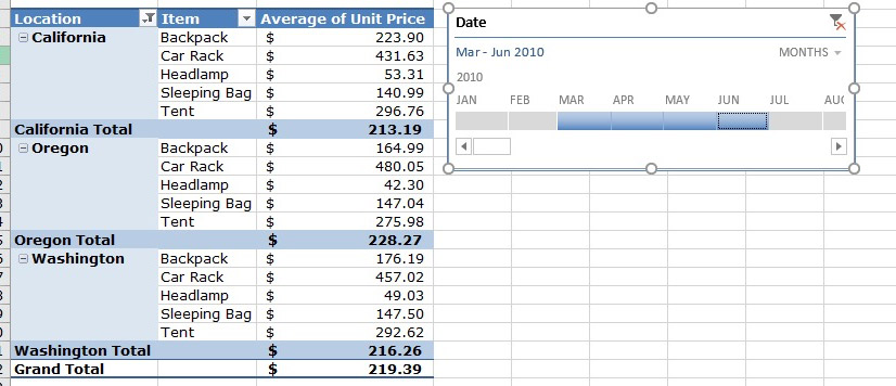
Once the timeline is inserted, you can click and drag the handles in the timeline to change what's included as a part of the PivotTable.

You can change the way your Timeline works by clicking on the dropdown box in the lower right corner. Instead of the timeline showing specific dates, you can change the timeline to show data based on the quarter or year, for example.

3. Tabular View

Excel's default PivotTable view looks kind of like a waterfall; as you drag more levels of fields into the rows box, Excel creates more "layers" in the data.

The problem is that PivotTables in the standard view are difficult to write formulas on. If you have your data in a PivotTable, but you want to view it more like a traditional spreadsheet, you should use tabular view for your PivotTable.

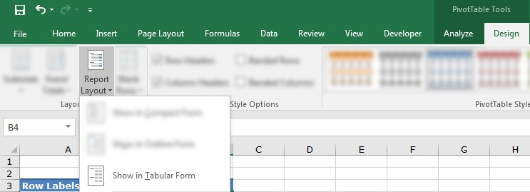
Why should you use Tabular View? Putting your PivotTable data in the classic, table style view will allow you write formulas on the data more easily, or paste it in a separate report.

For me, it's easier to use the tabular view in Excel most of the time. It looks more like a standard spreadsheet view and feels easier to write formulas and work with the data inside of it. I could also take this view and paste it into a new tab more easily.

4. Calculated Fields

Calculated fields are a way to add a column to your PivotTable that isn't in your original data. You can use standard math operations to create entirely new fields to work with. Take two existing columns and use math to create entirely new ones.

Let's say that we have sales data in a spreadsheet. We have the number of items sold, and the selling price for each item. This is the perfect time to use a calculated field to calculate the total of the order.

To get started with calculated fields, start off by clicking inside of a PivotTable and find then click Analyze on the ribbon. Click on the Fields, Items & Sets menu, and then choose Calculated Field. 

In the new pop up window, start off by giving your calculated field a name. in my case, I'll name it Total Order. A total order price is the quantity times the price of each unit. Then, I'll double click on the first field name (quantity) in the list of fields in this window.

After I've added that field name, I'll add the multiplication sign, * , and then double click on the total quantity. Let's go ahead and press OK. 

Now, Excel has updated my advanced PivotTable with the new calculated field. You'll also see the list of PivotTables in the list of fields, so you can drag and drop it anywhere in the report as you need it.

If you don't want to use math on two columns, you can also type your own arithmetic values in the calculated field. For example, if I wanted to simply add 5% sales tax for each order, I could write the following calculated field:

Basically, calculated fields can contain any of the standard math operators, such as addition, subtraction, multiplication and division. Use these calculated fields when you don't want to update the original data itself.

5. Recommended PivotTables

The Recommended PivotTables feature is so good that it feels like cheating. Instead of spending time dragging and dropping your fields, I find myself starting with one of the Recommended configurations.

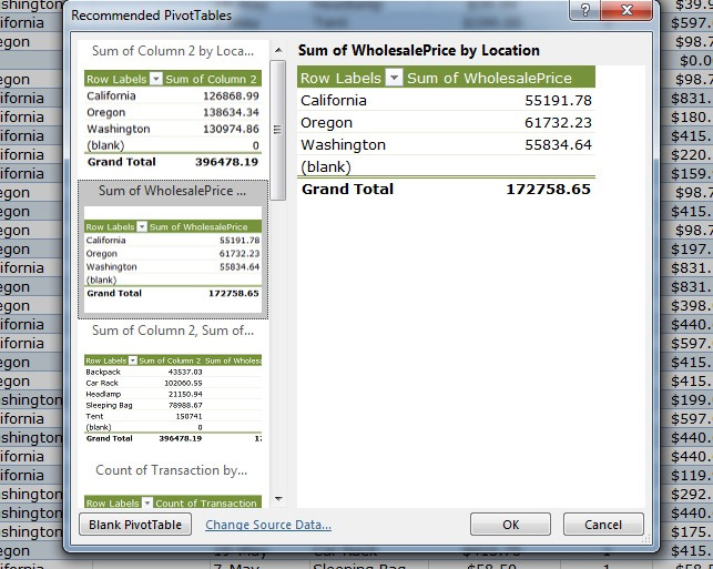
This feature is so easy to use that there's not much to say. You can use it to make advanced Pivot Tables in Excel quickly. Simply highlight your data, browse to the Insert tab on Excel's ribbon, and choose Recommended PivotTables.

The pop-up window features a litany of options for creating a PivotTable from your original data. Click through the thumbnails on the left side of this window to view the Recommended PivotTable options Excel generated.

Even though this is an advanced feature that not many users think about, it's also a great tool for starting with PivotTables. There's nothing stopping you from modifying the PivotTable by changing the fields on your own, but this is a time-saving starting point.

I also like this feature as a way to explore data. If I don't know what I'm looking for when I'm starting to explore data, Excel's Recommended PivotTables are often more insightful than I am!

Recap and Keep Learning (With More Excel Tutorials)

This advanced Excel tutorial helped you dive deeper into PivotTables, one of my favorite features to analyze and review an Excel spreadsheet. I use PivotTables to find meaning in large sets of data, which I can make good decisions from and take action.  

These tutorials will help you advance your Excel and PivotTable skills to the next level. Check them out:

• ExcelZoo has a great roundup of PivotTable techniques in their article, 10 Tutorials to Master PivotTables.
  
  


• We at Envato Tuts+ have covered PivotTables with a beginner's tutorial, How to Create Your First PivotTable in Microsoft Excel.


• For a more basic introduction to Microsoft Excel, check out our learning series How to Make and Use Excel Formulas (Beginner Bootcamp).

What do you still want to learn about PivotTables? Let me know about your ideas or questions in the comments below this tutorial.