Introduction to Linear Regression Algorithm with Example

In this article, we will learn about the linear regression algorithm with examples. First, we will understand the basics of linear regression algorithm, and then we will look at the steps involved in linear regression and finally an example of linear regression.

Regression is a supervised learning technique for determining the relationship between two or more variables. Regression fits a line or curve that passes through all the data points on a target-predictor graph in such a way that the vertical distance between the data points and the regression line is minimum. Regression is mainly used for prediction, time series analysis, forecasting, etc. There are many types of regression algorithms like linear regression, multiple linear regression, logistic regression, and polynomial regression.

Linear regression is a statistical method that is used for prediction based on the relationship between the continuous variables. In simple words, we can say that linear regression shows the linear relationship between the independent variable (X-axis) and the dependent variable (Y-axis), consequently called linear regression. If there is a single input variable (x), such linear regression is calledsimple linear regression. And if there is more than one input variable, such linear regression is calledmultiple linear regression.

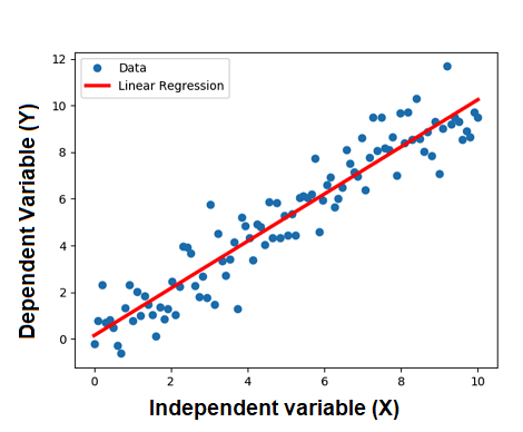
The linear regression model depicts the relationship between the variables as a sloped straight line as shown in the graph below. When the value of x (independent variable) increases, the value of y (dependent variable) is likewise increasing. In linear regression what we do is find a best fit straight line similar to the red line shown in the graph that fits the given data points best (i.e. with minimum error).

Mathematically we represent a linear regression as,

y = a + bx, for simple linear regression

y = a+ b1x1 + b2x2 + b3x3 + for multiple linear regression

Sometimes these equations are called hypothesis functions.

where,

a = intercept of the line or bias

b, b1, b2, = liner regression factor or scale factor or weights

x, x1, x2, = independent variables

y = dependent variable

During a linear regression analysis, we are given Xs and Y as training data and we have to obtain the intercepts (a), and regression factors (b, b1, b2,). Once we get the suitable value of intercepts and regression factors they can be used to predict the value of y for the input value of x.

We will consider simple linear regression from now onwards for simplicity.

A linear line showing the relationship between the dependent and independent variables is called aregression line. On the basis of the relationship between the independent and dependent variables, the regression line can be of two types.

Negative Linear Relationship:

If the dependent variable decreases on the Y-axis and the independent variable increases on the X-axis, then such a relationship is called a negative linear relationship.

In this condition, the equation will be, y = -a + bx

Positive Linear Relationship:

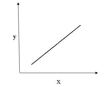
If the dependent variable increases on the Y-axis and the independent variable increases on X-axis, then such a relationship is termed a positive linear relationship.

In this condition, the equation will be, y = a + bx

How to find the best-fit line:

As we have mentioned earlier, the main motive of linear regression is to find the best fit line for the given data points. And the process of finding this best fit line is called learning of linear regression. Finding the best fit line means getting the best values for a and b based on the given dataset. The best fit line should have minimum error (i.e. the error between the predicted values and actual values should be minimized).

Cost function:

Cost functions are the error measuring functions that tell how the linear regression model is performing. It compares the predicted value of y with the actual value of y for the same input. There are various types of cost functions there. You can read about them here. From those, typically for the linear regression analysis, we use Mean Squared Error (MSE).

Where Ti is the actual/true value, Yi is the predicted value and n is the total number of data.

Gradient Descent:

In order to get the best-fit line, we have to find the suitable value of a, and b so that the cost function is minimum. To minimize the cost function we use a gradient descent algorithm. Gradient Descent is an iterative algorithm. The idea behind this algorithm is that we start with random values of a, and b and iteratively update the values such that the cost function is minimized. To read in detail about the gradient descent algorithm visit this.

Steps involved in Linear Regression Algorithm

Since we have covered the basic concepts now lets look at the steps involved in the linear regression algorithm.

1. Prepare the given data. Read more from here.
2. Decide the hypothesis function (i.e. for simple linear regression, y = a + bx is the hypothesis function )
3. Initialize a, and b with some random values.
4. Update the parameters a, and b using gradient descent algorithm i.e.
   1. Calculate y_predicted, y_predictedi = a + bxi
   2. Calculate cost function,
      1. 
   3. Compute the gradient of cost function with respect to parameters (dJ/da, dj/db)
   4. Update a and b using that gradient:
      • a = a lr*( dJ/da)
      • b = b- lr*( dJ/db), lr is learning rate.
   5. Repeat from steps I to iv until the desired result is obtained (i.e. cost function is minimized)

5. Once the gradient descent is completed we will get updated values of a, and b for which the cost function is minimum. And line corresponding to those values will be the best fit line.

The steps will be similar for the multiple linear regression.

Linear Regression Example

As mentioned earlier in the introduction section that this article will be learning linear regression algorithm with an example, now its time to do so. We will look at an example that you can find in scikit-learn.org.

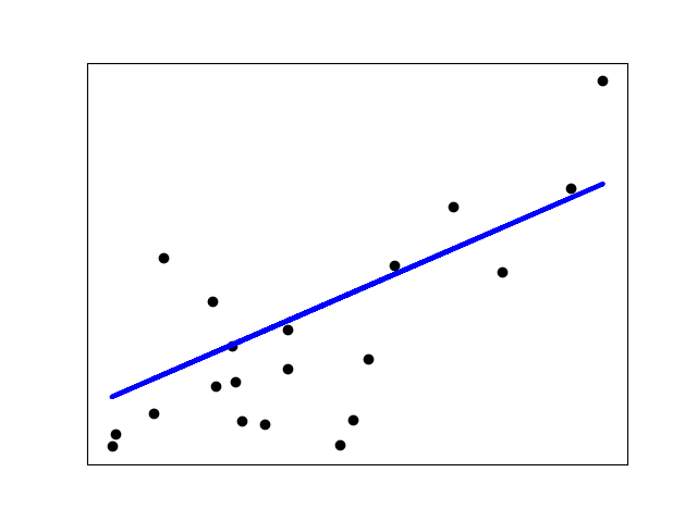
For this linear regression example, the diabetes dataset is used. You can find more about it from here. The example below uses only the first feature of thediabetesdataset, in order to illustrate the data points within the two-dimensional plot. The straight line can be seen in the plot, showing how linear regression attempts to draw a straight line that will best minimize the residual sum of squares between the observed responses in the dataset, and the responses predicted by the linear approximation.

The coefficients, residual sum of squares, and the coefficient of determination are also calculated.

# Code source: Jaques Grobler# License: BSD 3 clauseimport matplotlib.pyplot as pltimport numpy as npfrom sklearn import datasets, linear_modelfrom sklearn.metrics import mean_squared_error, r2_score# Load the diabetes datasetdiabetes_X, diabetes_y = datasets.load_diabetes(return_X_y=True)# Use only one featurediabetes_X = diabetes_X[:, np.newaxis, 2]# Split the data into training/testing setsdiabetes_X_train = diabetes_X[:-20]diabetes_X_test = diabetes_X[-20:]# Split the targets into training/testing setsdiabetes_y_train = diabetes_y[:-20]diabetes_y_test = diabetes_y[-20:]# Create linear regression objectregr = linear_model.LinearRegression()# Train the model using the training setsregr.fit(diabetes_X_train, diabetes_y_train)# Make predictions using the testing setdiabetes_y_pred = regr.predict(diabetes_X_test)# The coefficientsprint('Coefficients: n', regr.coef_)# The mean squared errorprint('Mean squared error: %.2f'      % mean_squared_error(diabetes_y_test, diabetes_y_pred))# The coefficient of determination: 1 is perfect predictionprint('Coefficient of determination: %.2f'      % r2_score(diabetes_y_test, diabetes_y_pred))# Plot outputsplt.scatter(diabetes_X_test, diabetes_y_test,  color='black')plt.plot(diabetes_X_test, diabetes_y_pred, color='blue', linewidth=3)plt.xticks(())plt.yticks(())plt.show()

Output:

Coefficients: [938.23786125]Mean squared error: 2548.07Coefficient of determination: 0.47