Build a simple travel planning application using graph algorithms, Cypher & Python

Introduction

Backpacking is a great way to explore the world on a budget. With its great transportation network, affordable accommodations, and thousands of attractions, Europe is the perfect travel destination for backpackers.

In this tutorial, you will learn how to build a simple travel planning application leveraging Memgraph, Cypher, and Python. You will learn how to work with a graph database and how to query it using a Python language driver. You will also learn how to leverage popular graph algorithms including breadth-first search (BFS), and Dijkstra's algorithm.

Prerequisites

To follow along, you will need the following:

• A machine running Linux.
• A local installation of Memgraph. You can refer to the Memgraph documentation.
• The Python Memgraph Client.
• A basic knowledge of the Python programming language. We will be using Python 3 for this tutorial.
• Basic knowledge of the Cypher query language.

Step 1 Defining The Data Model

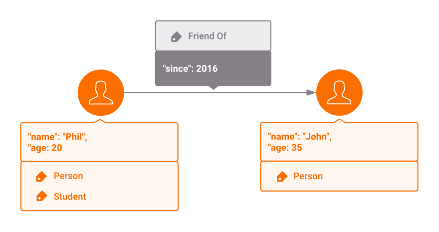
First, we have to define the data model we will be using to build your application. One of the most common data models used for graph analytics is the Lable Property Graph (LPG) model. This model is defined as a set of vertices(aka nodes) and edges(aka relationships) along with their properties and labels.

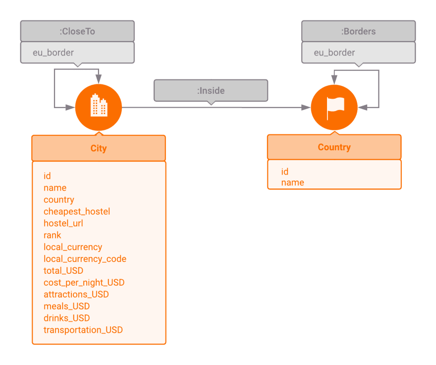
In this tutorial, you will be using the European Backpacker Index (2018) dataset containing information about 56 cities located in 36 European countries. Your model will contain two vertices types City and Country, and three edges of types Inside, CloseTo, and Borders along with a few properties such as names, rankings, local currencies, etc.

Now that you have defined your data model, the next step is to import the data to Memgraph.

Step 2 Importing Data Into Memgraph with Cypher and Python

In order to import the data into Memgraph, you will be using Cypher queries through the Python client pymgclient.

The pymgclient is a Memgraph database adapter for Python programming language compliant with the DB-API 2.0 specification described by PEP 249.

Cypher is a declarative query language considered by many to be the industry standard when it comes to working with property graph databases.

Before getting started, you have to install the pymgclient. This will allow you to connect to Memgraph and run your queries. To do this, we will run the following command:

pip install pymgclient

Now that we have the pymgclient installed, we're ready to import it and connect it to the Memgraph database. To do this, we will use the following Python code:

import mgclient# Connect to the databaseconnection = mgclient.connect(    host='127.0.0.1',    port=7687,    sslmode=mgclient.MG_SSLMODE_REQUIRE)connection.autocommit = True

Now that our python client is connected to the Memgraph, we're ready to start running our queries. In order to accelerate the data import, we create indexes on id property of the City and Country vertices. This will help Memgraph quickly find cities and countries when creating edges. Note that we could create the index on another property such as name and we would achieve the same result.

[NOTE] A database index essentially creates a redundant copy of some of the data in the database to improve the efficiency of searches for the indexed data. However, this comes at the cost of additional storage space and more writes, so deciding what to index and what not to index is an important decision.

In order to create our indexes, we will execut the following queries:

connection.cursor().execute("""CREATE INDEX ON :City (id)""")connection.cursor().execute("""CREATE INDEX ON :Country (id)""")

Now that our indexes are created, we will begin importing our, starting with countries. To do this, we will run the following queries.

As you can see, this query uses the CREATE clause to create a vertex with one label, Country, and 2 properties, id and name.

Next, we will add the City nodes with all of their properties such as the local currency, the average price of meals and drinks, the cost of transportation, etc. To do this, we will use the following queries.

As you can see, this query uses the same CREATE clause to create nodes with label City, and 14 different properties.

Now that we have created all the nodes in our graph, we're ready to start adding edges. To do this, we will run the following queries.

In this query, we first use the MATCH clause to get the two City nodes between which we will be creating an edge and then use the CREATE clause to create an edge of label CloseTo and a property eu_border with can have a value of True or False.

Congrats! You have now imported all your dataset to Memgraph. You are now ready to start executing queries and algorithms.

Step 3 Running Simple Cypher Queries with Python

To get started, we can run some simple queries such as getting the top 10 cities with the cheapest hostels. To do this, you would run the following query:

cursor = connection.cursor()cursor.execute("""MATCH (n:City)RETURN n.name, n.cheapest_hostel, n.cost_per_night_USD, n.hostel_urlORDER BY n.cost_per_night_USD LIMIT 10""")print(cursor.fetchall())

This query matches all vertices with label City and returns the city name, the name of the cheapest hostel, the cost per night for that hostel, and the hostel URL. It then ranks the results based on the cost per night of the cheapest hostel, and return the top 10 results.

What if you're visiting Italy to know which cities are recommended for backpackers and which is the cheapest hostel for every one of them. To get the answer, you will run the following query:

cursor = connection.cursor()cursor.execute("""MATCH (c:City)-[:Inside]->(:Country {name: "Italy"})RETURN c.name, c.cheapest_hostel, c.total_USDORDER BY c.total_USD;""")print(cursor.fetchall())

As you can see the query resembles the one we used before, but instead of matching all the cities, we're only matching the ones that are connected to Italy through the edge of type Inside

Step 4 Using the Breadth-First Search Algorithm to Find and Filter Paths

Although these queries give us some interesting insights and results, they are not something graph databases are particularly interesting for. Graph databases become valuable when we start asking more complex questions that involve traversing an arbitrary number of edges. These types of pathfinding queries can become problematic for traditional databases as they often require multiple joins.

Say you want to travel from Spain to Russia, but you want to pick the route that crosses the least amount of borders. This is where a graph algorithm like breadth-first search (BSF) comes in handy. To get your answer, you will use the following query:

cursor = connection.cursor()cursor.execute("""MATCH p = (n:Country {name: "Spain"})          -[r:Borders * bfs]-          (m:Country {name: "Russia"})UNWIND (nodes(p)) AS rowsRETURN rows.name;""")print(cursor.fetchall())

This query evaluates all possible paths between Spain and Russia using the edges of type Borders, counts the number of border crossings for each path, and returns the path with the lowest number of border crossings.

What if you want to filter paths based on certain criteria? Say you want to drive from Bratislava to Madrid and want to plan your route to minimize the number of stops. You also want to only visit countries that have the Euro as a local currency since that's the only currency you have left. To do this, you will use the following query:

cursor = connection.cursor()cursor.execute("""MATCH p = (:City {name: "Bratislava"})          -[:CloseTo * bfs (e, v | v.local_currency = "Euro")]-          (:City {name: "Madrid"})UNWIND (nodes(p)) AS rowsRETURN rows.name;""")print(cursor.fetchall())

As you can see, we added a special syntax to the query (e, v | v.local_currency = "Euro"). This is called a filter lambda function. The filter lambda takes an edge symbol e and a vertex symbol v and decides whether this edge and vertex pair should be considered valid in the breadth-first expansion by returning true or false (or Null). In this example, the lambda function is returning true if the value of the property of type v.local_currency of the city vertex v is equal to Euro. Once the best path is identified, the query returns the nodes(p) as a list, and the UNWIND clause unpacks the list into individual rows.

Step 5 Using Dijkstras Algorithm to find the Shortest Path

So far, you used the breadth-first search algorithm to find the path that crossed the smallest number of edges. But what if instead, you wanted to find the shortest path taking into consideration the price of accommodations for every city you would visit on your path? In other words, what if you want to find the shortest cheapest path? This is where the breadth-first search algorithm reaches its limit. BFS will accurately calculate the shortest path only if all edges and vertices either have no weight or have the same weight.

When it comes to finding the shortest path in a graph where edges and vertices don't have the same weight, you will need to use Dijkstras algorithm.

For example, let's say you want to travel from Brussels to Athens and you're on a tight budget. In order to find the cheapest route, you would use the following query:

cursor = connection.cursor()cursor.execute("""MATCH p = (:City {name: "Brussels"})          -[:CloseTo * wShortest (e, v | v.cost_per_night_USD) total_cost]-          (:City {name: "Athens"})WITH extract(city in nodes(p) | city.name) AS trip, total_costRETURN trip, total_cost;""")print(cursor.fetchall())

As you can see, the syntax is almost identical to our BFS queries. We use the weighted shortest path wShortest and specify thecost_per_night property type as our weight. The weight lambda indicates the cost of expanding to the specified vertex using the given edge v.cost_per_night_USD, and the total cost symbol calculates the cost of the trip. The extract function is used to only show the city names. To get the full city information, you would return nodes(p).

Conclusion

There you have it! You just learned how to build a simple travel route planning application using a graph database, Cypher, and Python. You also learned how to use the breadth-first search algorithm and Dijkstras algorithm to navigate a complex network of interconnected data and filter your results using the powerful and flexible lambda function.