How to Use the Excel VLOOKUP Function - With Useful Examples

What is a VLOOKUP in Excel?

A VLOOKUP, short for "vertical lookup" is a formula in Microsoft Excel to match data from two lists. Instead of jumping between spreadsheets and typing out your matching data, you can write a VLOOKUP formula to automate the process.

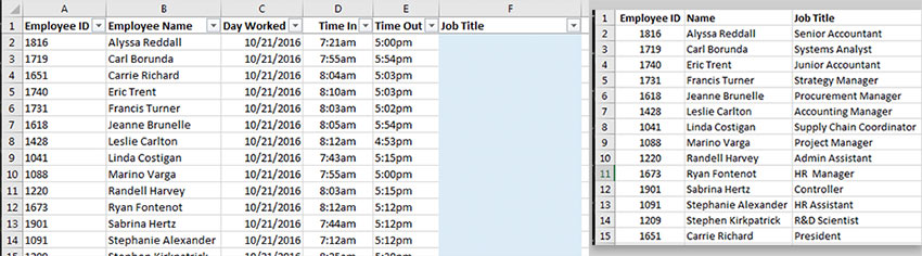
On the left (in the image above), we have employee shift information. We want to add the employee's job title to the shift data. With a separate list of employees and their job titles, we can write a VLOOKUP formula to pull in the title from a lookup list.

A successful VLOOKUP needs three things:

• A primary key in each list that you can use to match your data up. The two lists need to share at least one piece of data in common (in the Excel VLOOKUP example above, this is the employee ID)


• A Lookup List, which contains your "database", or basically the information (the list of employee job titles)


• Your data, which you want to pull a match into (the shift data)

Quick Example of an Excel VLOOKUP Formula in Action

VLOOKUP is a Microsoft Excel formula that's essential for working with multiple sets of data. In this tutorial, I'll teach you how to master and use it.

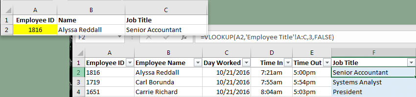
Using the example above, I've now written a VLOOKUP formula that looks up the employee's ID and inserts the job title into the shift data. Because both sheets have an employee ID, Excel can lookup the matching job title. The best part of VLOOKUP is that I can now drag the same formula down and it will look up each unique job title.

Free Excel Spreadsheet Download 

Before we move on, make sure to Download the free Attachment to follow along. It's an example spreadsheet workbook that I created, which we'll use to walk through this tutorial.

Watch and Learn: VLOOKUP

For the fastest way to learn the basics of the VLOOKUP formula, check out the screencast below. The video walks through several examples of the VLOOKUP formula, using the example workbook.

Keep reading to walk through the written instructions, and learn some additional techniques that aren't covered in the screencast.

How to Use VLOOKUP in Excel: Walk Through 

Use the tabs "Ingredient Orders" and "Supplier List" for this Excel VLOOKUP example.

Let's say that we manage a restaurant and are placing our weekly orders to suppliers. The chefs have given us a list of ingredients to order, and we need to insert information about the supplier.

There are three pieces we need to add for each order:

• The Supplier Name


• The Supplier Phone Number


• The Supplier Delivery Day

In this workbook, there are two tabs:

• 
  Ingredient Orders - contains the list of ingredient requests from our chefs.


• 
  Supplier List - contains information about the suppliers, such as the supplier name and phone number.
  
  

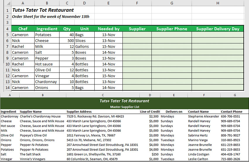
The common field between the two tables is the Ingredient tab. Let's use it to lookup each of the three fields and add it to the order list.

Step 1: Start Our Excel VLOOKUP Formula

On the Ingredient Orders tab, let's click in the first blank Supplier cell, F5, and press the equals sign to start the VLOOKUP formula. Then, type " VLOOKUP( " to start the formula.

 =VLOOKUP(

Remember that our primary key—the piece of data that appears in both lists—is the ingredient, so we'll use it for the lookup. Either click on cell B5, or type it into the formula. Next, add a comma after "B5" so that we can enter the next part of the formula. 

=VLOOKUP(B5,

Now, we need to give the formula our lookup list. With the formula still open, click on the Supplier List tab. Now, click on cell A3, and click and drag to highlight and select A3 to G13, the whole lookup table. Make sure and press the F4 key on your keyboard to make the formula an absolute reference (more on this later). Finally, enter another comma.

After you enter the comma for the lookup cell, switch tabs and point Excel to the lookup list. Click and drag between cells A3 and G3 to select the data to lookup from. Make sure and press F4 on your keyboard during this step to create an absolute reference, which will lock in the cells to use for the lookup.

=VLOOKUP(B5,'Supplier List'!$A$3:$G$13,

Next up, we'll need to tell Excel which column to pull from. Remember that our first item to insert is the Supplier name, which is in the second column of the lookup list. Add the number 2 to the formula to pull from the second column of the lookup, and another comma.

=VLOOKUP(B5,'Supplier List'!$A$3:$G$13,2,

Finally, we'll add FALSE for an exact lookup, and then close the parentheses:

=VLOOKUP(B5,'Supplier List'!$A$3:$G$13,2,FALSE)

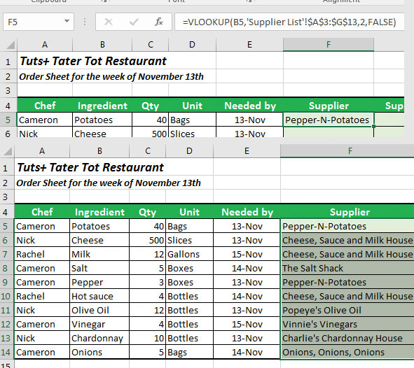
The good news is that we don't need to rewrite this same formula over and over—just double-click in the lower right corner of cell F5 (you can see the small green box on the corner of the cell) to extend the formula down (as shown above).

The formula is working perfectly! Okay, now let's move on to pulling in the data for the other two fields: the supplier phone number and delivery day.

Step 2: Pull More Data With Our VLOOKUP

Because we used an absolute reference, we can basically reuse the same formula we wrote with a minor tweak. Let's add in the Supplier Phone Number next.

We'll start off by copying and pasting cell F5 (our Supplier cell) to cell G5. I typically just use the keyboard shortcuts Ctrl + C and Ctrl + V to copy and paste the entire cell. At first, this won't be working, and you'll see an N/A in the cell. 

It's much easier to copy and paste our formula into another cell, but it requires some tweaking. At first, Excel will be looking to cell C5 for the lookup, but we need to adjust it to "B5" in the formula bar. Once we do that, the lookup will be working - almost.

We'll need to go up to the formula bar, and change the first part of the formula from C5 back to B5. When we moved the formula over by one column, Excel updated other parts of the formula. We were getting an "N/A" because Excel was attempting to match the quantity (Column C) to our lookup list, but our lookup list doesn't include the quantity.

So far, our formula so should be:

=VLOOKUP(B5,'Supplier List'!$A$3:$G$13,2,FALSE)

However, notice in the screenshot above that we're pulling the wrong bit of data into the "Phone" column. We're still pulling the second column in the lookup list with the "2" in the formula. We need to change this to the column number with our supplier's contact phone.

Step 3: Fix VLOOKUP N/A Error Issue

Let's go back and check out the lookup list. You'll notice that the phone number is in the 7th column in the lookup list. Let's go back to our Excel formula and update the lookup to pull from the 7th column.

All that we need to do is update the column section of our lookup list from a "2" to a "7" and it now works great!

Our final formula for the supplier phone number lookup:

=VLOOKUP(B5,'Supplier List'!$A$3:$G$13,7,FALSE)

Step 4: Add Another Column to Finish Our VLOOKUP Formula

Finally, let's work in the Supplier Delivery Day column. Copy and paste cell G5 to cell H5. Again, we'll need to fix our formula by changing C5 back to B5 to use the ingredient as the primary key. Then, just update the "7" to a "5" to use the 5th column from our lookup table.

Our final formula for the supplier delivery day:

=VLOOKUP(B5,'Supplier List'!$A$3:$G$13,5,FALSE)

That's it! We wrote basically one formula and tweaked it to pull in every bit of data we need to place our next order.

Troubleshooting VLOOKUP

So, you've written the VLOOKUP formula following the instructions step-by-step, but it's still not working. Excel takes things pretty literally, so we need to be careful with the data and the VLOOKUP formula. Let's take a look at several ideas for correcting a VLOOKUP formula that's just not working.

1. Multiple Matches

One of the most common issues with VLOOKUP is when there are multiple matches in your lookup list. When you're using a VLOOKUP, it will match to the first item that's in the list.

The point of VLOOKUP is to look up a matching item against a list. The lookup list shouldn't contain duplicates for the primary key, the item that you're using to match. Otherwise, Excel gets confused and only shows you the first match.

2. Leading or Trailing Spaces

Another common issue is that our data might not actually match in Excel's eyes. Data with a space before it is said to have a "leading" space, while data with a space after it has a "trailing space."

If your matching piece of data has a space before or after it, Excel sees these two pieces of data as totally different, and won't return a match. Excel views "_Andrew", "Andrew_" and "Andrew" as three unique pieces of data that won't be matched in VLOOKUP.

If your data has leading or trailing spaces, use the TRIM function in Excel to clean it up. VLOOKUP should work great after using it to remove leading and trailing spaces.

3. Lock in Cell References

As you might know, you can drag a cell down by the handle to paste the formula into other cells. However, this sometimes breaks our VLOOKUP because the cell references change. 

As you pull the formulas down, it pulls the reference for the lookup table out of alignment. Suddenly, the lookup table is missing rows from the lookup table and our VLOOKUP isn't working.

The fix is to make the formula an absolute reference, so that when you drag the formula down, the list it's pointing to doesn't change. Click in the cell where you've written your VLOOKUP, and then click somewhere in the lookup list reference. Then, press F4 . You'll notice that the formula changes to include dollar signs.

Recap and Keep Learning

VLOOKUP is one of those essential formulas for being a productive Excel users. There's simply not enough time to manually look up data and re-type it over and over again, so formulas like VLOOKUP are important to learn.

• If you want to learn an assortment of more advanced Excel skills, check out Bob Flisser's 12 Techniques for Power Users tutorial. 


• Additionally, Bob's course Introduction to Spreadsheets is the perfect guide to getting started in Excel


• Sometimes, it helps to learn similar material from another resource. The Microsoft Office official documentation on the VLOOKUP formula is another great resource for mastering VLOOKUP.

If you're having any problems with using the VLOOKUP formula, feel free to leave a comment below for troubleshooting.