The theory behind Image Captioning

Introduction

One of the most challenging tasks in artificial intelligence is automatically describing the content of an image. This requires the knowledge of both computer vision using artificial neural networks, and natural language processing. This can have great impact in many different domains - be it to make it easier for visually impaired people of the community to understand the contents of the images on the web, or for tedious tasks like data labelling where data is in the form of images. In this article, we will walk through the basic concepts that are needed in order to create your own image captioning model.

Textual description of an image

In principle, converting an image into text is a significantly hard task. The description should not only contain the objects highlighted in the image but also the context of the image. On top of that the output has to be expressed in a natural language like English, German, etc., so a language model is also needed to complete the picture.

In the above image we see people on a vacation hiking on the foothills of a mountain range. Let us say that we want to generate a text describing this image. The image is used as input I and is fed to the model (called the Show and Tell model, developed by Google) which is trained to maximise the likelihood p( S | I ) of producing a sequence of words S = {S, S, ...., S}, where each word S comes from a given dictionary which describes the image accurately.
In order to process the input data, we use Convolutional Neural Networks (CNNs) as "encoders" and the output of the CNN is fed to a type of Recurring neural network called Long-Short Term memory (LSTM) network which is responsible for generating natural language outputs. Before describing the model, let us briefly look into CNNs and LSTM.

Convolutional neural networks

CNN is a type of neural network which is used mainly for image classification and recognition. As the name suggests, it uses a mathematical operation called convolution to process the data. The CNN consists of an input layer, single or multiple hidden layers, and an output layer. The middle layers are called hidden because their inputs and outputs are masked by the activation function.

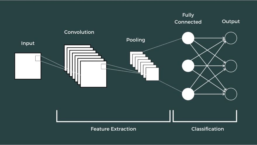
Convolutions operate over 3D tensors called feature maps with two spatial axes and a channel axis. The hidden layers (convolutional layers) are made up of multiple convolutions that scan the input data and apply filters to extract output feature. This output feature is also a 3D tensor which is passed through a non-linear activation function in order to induce non-linearity.
The output of the convolutional layers is passed through a pooling layer, which aggressively downsamples the feature maps and reduce computation complexity. Eventually, the output of the pooling layer is passed through a fully connected dense layer, which computes the final prediction.
Below is an example of how to instantiate a convolutional neural network in python:

from tensorflow.keras import layersfrom tensorflow.keras import modelsfrom tensorflow.keras import optimizersmodel = models.Sequential()model.add(layers.Conv2D(32, (3,3), activation='relu', input_shape=(120, 120, 10)))model.add(layers.MaxPool2D((2,2)))model.add(layers.Conv2D(64, (3, 3), activation='relu'))model.add(layers.MaxPooling2D((2, 2)))model.add(layers.Conv2D(128, (3, 3), activation='relu'))model.add(layers.MaxPooling2D((2, 2)))model.add(layers.Conv2D(128, (3, 3), activation='relu'))model.add(layers.MaxPooling2D((2, 2)))model.add(layers.Flatten())model.add(layers.Dense(512, activation='relu'))model.add(layers.Dense(1, activation='sigmoid'))model.compile(loss="binary_crossentropy",              optimizer=optimizers.RMSprop(learning_rate=1e-3),               metrics=['acc'])

Here we have assumed that the user already has the pre-processed input data. Let us assume that this data is split into training and test sets. In the next step, we can fit the model and save it.

fitting = model.fit_generator(            training_data,            steps_per_epoch=80,            epochs=25,            validation_data=validation_data,            validation_steps=70          )model.save("output_data.h5")

Long-short term memory

LSTM networks are type of recurrent neural networks that are well suited for modelling long-term dependencies in data. They are called "long-short term" because they can remember information for long periods of time, but they can also forget information that is no longer relevant.
RNN was a consequence of the failure of the feedforward neural networks.
Problems with feedforward neural networks?

• Not designed for sequences and time series
• Do not model memory - in the sense that they do not retain information from previous data points when processing new data.

RNNs solve this issue conveniently. The recursive formula defined as:

states that the new state at time 't' is a function of the old state at 't-1' and input at time 't'. This makes the RNNs different from other neural nets (NNs) since NNs learn from backpropagation and RNNs learn from backpropagation through time!

The output from this network is now used to calculate the loss.

In the image shown above, we describe a recurrent neural network which is run for - say - 100 time steps. Our aim is to compute the loss. Let us assume that at each state, out gradient is 0.01. As we go back a 100 time steps, the update in our weights is

The above image shows the functionality of the LSTM network. The important part is that the network can decide what information to discard and what to keep. This resolves the vanishing gradient problem that we face in a normal RNN.
Here is a simple implementation of the LSTM network in keras-

from tensorflow.keras.layers import LSTMfrom tensorflow.keras import modelsmodel = models.Sequential()model.add(Embedding(max_features, 32))model.add(LSTM(32))model.add(Dense(1, activation='sigmoid'))model.compile(optimizer='rmsprop',              loss='binary_crossentropy',              metrics=['acc'])model_fitting = model.fit(input_train, y_train,                    epochs=30,                    batch_size=128,                    validation_split=0.2)

Back to the textual description

Now that we have gone through the concepts of the tools required, it is understood that using CNNs to process the image inputs and LSTM for natural language output we can build rather accurate models to generate image captions. For that, use a CNN as an encoder, by pre-training it first for image classification and using the last hidden layer as an input to the RNN "decoder" that generates sentences.
The model is trained to maximise the likelihood of generating correct description given the image which is given as:

where are the parameters of the model, I is the input image, and S is correct word. The loss is described as the negative log likelihood of the correct word at each step:

Once the loss is minimized and the likelihood maximized, we have to consider the epoch where the validation loss is minimum. And tada! We have our model ready. All you would have to do is to input the images and the expected output should be a sentence describing that image.

This article is more about the in-depth knowledge of the tools used to build this use case. Once you are proficient enough, you can create your own use case and build your own models for it.

Citations:

• A neural image caption generator.
• What is LSTM? - IBM Technology
• Deep Learning using python.