Analysis of classification models on NASA Active Fire data.

This article is based on the prediction of the type of forest fire detected by MODIS in India (year 2021) using Classification algorithms.

Checkout the code here (don't forget to give it an upvote!)

• MODIS (or Moderate Resolution Imaging Spectroradiometer) is a key instrument aboard the Terra and Aqua satellites.
• It helps scientists determine the amount of water vapor in a column of the atmosphere and the temperature thus helping detect forest fires.

We are trying to predict the type of forest fire which can be a hurdle considering the vast vegetation and forest area in different parts of the world with the help of Active Fire Data provided by NASA.

You can find all the datasets here

This report highlights the ML algorithms used and its analysis, while in the end we discuss the best suited algorithm for the prediction.

About the dataset used:

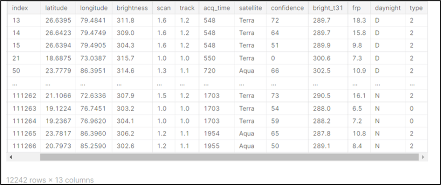
MODIS Active Fire Data of India year 2021:

It consists of:

• latitude: Latitude of the fire pixel detected by the satellite (degrees)
• longitude: Longitude of the fire pixel detected by the satellite (degrees)
• brightness: Brightness temperature of the fire pixel (in K)
• scan: Area of a MODIS pixel at the Earths surface (Along-scan: S)
• track: Area of a MODIS pixel at the Earths surface (Along-track: T)
• acq_time: Time at which the fire was detected
• satellite: Satellite used to detect the fire. Either Terra(T) or Aqua(A)
• instrument: MODIS (used to detect the forest fire)
• confidence: Detection confidence (range 0-100)
• bright_t31: Band 31 brightness temperature of the pixel (in K)
• frp: Fire radiative power (in MW- megawatts)
• daynight: Detected during the day or night. Either Day(D) or Night(N)
• type: Inferred hot spot type:
  • 0= presumed vegetation fire
  • 1= active volcano
  • 2= other static land source
  • 3= offshore

We will be predicting the Type feature using several classification models.

Analyzing the classes:

• Since the type 3 has very little data to work with, we can drop it so that it doesn't affect our model.
• For type 0 and 1, there is a slight imbalance that we have to deal with. We can use StratifiedShuffleSplit library of sklearn for the same.

StratifiedShuffleSplit helps distribute the classes evenly between the training and testing data

Correlation between the features:

• Very few of the features are highly correlated, we can drop them to avoid duplicity.
• After some pre-processing and feature engineering, we can now apply our classification algorithms.

Machine Learning Algorithms

We make the use of 3 Machine Learning Algorithms:

• Logistic Regression
• KNN (Classifier)
• XG Boost (Classifier)

1. Logistic Regression:

Here, we use the liblinear solver (since we have a small dataset) with l2 regularization which doesnt make much of a difference without it, but it gives us lesser computational complexity.

You can learn more about it here.

Confusion Matrix:

The confusion matrix for Logistic Regression depicts the following:

• No type 0s are predicted incorrectly.
• 167 type 2s are predicted as 0, which means almost 20% of the type 2s predicted incorrectly.

Overall classification report:

The final accuracy of Logistic Regression Model is 93%.

• It can be noted that the recall for type 0 for logistic regression is 1.0, that is 100% of type 0s are correctly predicted while only 80% of type 2s are predicted correctly.
• This can occur due to fairly higher number of type 0s than type 2s in the dataset.

2. K Nearest Neighbours:

To select the K value, we first iterate between a number of K values, and find the accuracy rate for each K value and plot the values against the accuracy.

• This graph depicts that K=2 gives us the maximum accuracy, after which the accuracy is consistent. Hence, we use K=2 to fit our model.

Overall Classification report:

Final accuracy for KNN is 95%

Let's take a look at the confusion matrix:

The number of type 0s predicted for KNN incorrectly are higher than that of Logistic Regression that has a recall of 1.0 for type 0, but since the recall for type 2 is higher (87%) than that of logistic regression (81%), hence the f1 score for KNN increases.

3. XG Boost:

• I thought of choosing a Boosting algorithm over Bagging, looking at the performance of the first two algorithms, there was a need to decrease the bias.
• Since the dataset has around 12,000 rows, overfitting isnt a problem. Hence a Bagging algorithm wouldnt have been much of a help.
• For XG Boost, to find the best estimator, like we did for KNN, we will first iterate over a list of number of trees for our boosting model and plot it on a graph with the error.

• As shown in the graph above, for n_estimators = 200, lowest error is shown.

• To make the best use of all the hyperparameters, we cannot possibly iterate over the combinations of all possible parameters, hence we make the use of the library GridSearchCV library provided by sklearn, to find the best estimator.

To learn more- GridSearchCV

• We get max_features=4 and n_estimators=200 (As calculated by us above)
• Therefore, we use these parameters to get the accuracy of our model.

Overall classification report:

The classification report for XG Boost shows us the best results so far, with an accuracy of 98% and a higher precision and recall.

Confusion Matrix for XG Boost:

Less than 2% or readings predicted incorrectly.
Final accuracy for XG Boost is 98%.

Analysis

• Logistic Regression had a 100% recall for type 0, it could not perform well to predict the type 2 class with almost 20% error rate.
• KNN overcame the shortcomings of Logistic Regression giving a higher recall, but still suffered from high bias, hence the accuracy increased but at a smaller.
• Since the distribution of the features is very close to each other, it is hard to come up with stronger assumptions for our prediction.
• XG Boost on the other hand had undoubtedly the overall highest results, with a good f1 score and 98% accuracy, this can be implied due to the ensemble techniques of XG Boost, the nature of it being able to correct the mistakes of the weaker model, makes it stronger than Logistic Regression and KNN.

Conclusion:

It is apparent that the performance of XG Boost is far ahead from that of Logistic Regression and KNN. It will be the best suited algorithm with an accuracy of 98% for our prediction on the MODIS Forest Fire dataset.

Kaggle Notebook

Dataset