Sources Contact Advanced Search Tutorials

An Interest In:

Web News this Week

Search Archive

Some of Our Sources

View All Sources

Help Webnuz

Referal links:

October 21, 2022 07:26 am GMT

AI learning how to land on the moon

Welcome everyone to this post where I teach an AI how to land on the moon.

Of course I am not talking about the actual moon (although I wish I was), however I am talking about a simulated environment instead (OpenAI's Lunar Lander Gym environment)

Reinforcement Learning

I recently came across an article about DeepMind's AlphaTensor.

You can read about it here

AlphaTensor learnt how to multiply two matrices together in an extremely efficient way, managing to complete multiplications in fewer steps than Strassen's algorithm (the previous-best algorithm).

Reading this article inspired me to read into an area of machine learning I did not know much about - reinforcement learning. DeepMind has built several other very impressive AIs, which were all trained using reinforcement learning algorithms.

What is reinforcement learning?

Reinforcement learning concerns learning the best actions to take in certain situations in an environment in order to achieve a certain goal. For example, in a game of chess, RL algorithms would learn what piece to move and where to move it, given the state of the game board and the goal of winning the game.

RL models learn purely from their interactions in an environment. They are given no training dataset with what are the best actions to take in a given situation. They learn everything from experience.

How do they learn?

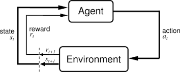
An agent is anything that interacts with an environment by observing it and taking actions based on those observations.

For each action the agent takes in an environment, the agent is given a reward which indicates how good that action was, given the observation and the aim of the agent in the environment.

RL algorithms improve the performance of these agents essentially through trial and error. They initially perform random actions and see what rewards they get from them. They then can develop a policy over time based on these action-reward pairs. A policy describes the best actions to take in given situations, with the goal of the environment kept in mind.

There are several algorithms available for developing a policy.

For this project, I used a DQN (Deep Q-Network) to develop a policy.

Q-Values and DQNs

DQNs are neural networks that take in the state of the environment as input and output the q-values for each possible action that the agent can take. It describes the agent's policy.

There is no fixed model architecture for DQNs. It varies from environment to environment. For example, an agent playing an Atari game might observe the environment through a picture of the game. In the case, it would be best to use convolutional layers as part of the DQN architecture. Using a simple feedforward neural network would work fine with other environments, such as the lunar lander environment in OpenAI's Gym.

Q-values measure the expected future rewards when taking that action, assuming that the same policy is followed in the future. When an agent is following a policy, it takes the action with the greatest q-value at the current state it's in.

The way DQNs are trained to determine accurate q-values will be explained as I go through the code.

DQNs are used when the action space in an environment is discrete i.e there is a finite number of possible actions an agent can take in an environment.

For example, if an environment involved driving a car, its action space would be considered discrete if the only actions allowed were to drive forward, turn left and right 10 degrees. Its action space would be continuous if actions involved specifying the angle of the steering wheel and the speed to travel at. This is because these can take an infinite number of values and, therefore, there an infinite number of actions.

Problem and Code

As I mentioned earlier, I am going to train an agent within OpenAI's Lunar Lander Gym environment.

The aim of the agent in this environment is to land the lander on its legs between the two flags.

The agent can take 4 actions:

Do nothing
Fire left engine
Fire right engine
Fire main engine

An observation taken from this environment is an 8-dimensional vector containing:

X coordinate
Y coordinate
X velocity
Y velocity
Angle of the lander
Angular velocity
2 Booleans describing whether each leg is in contact with the ground or not

The agent is rewarded as follows:

-100 points for crashing
+100 points for coming to rest
+10 points for each leg in contact with the ground
-0.3 points for each frame firing main engine
-0.03 points for each frame firing a side engine
+100 - 140 points for moving from top to the landing pad
The agent is considered to have solved the environment if it has collected at least 200 points in an episode.

episode - series of steps/frames that occur until some criteria for the environment to reset has been met (episode termination)

Episodes terminate if:

the lander crashes
the lander goes out of view horizontally

Training a DQN

An agent interacts with an environment by taking actions in it. For each step in the environment, the agent records the following into a replay memory:

The observation it took of the environment
The action it took from this observation
The reward it gained
The new observation of the environment
Whether the episode has terminated or not

The agent has an initial exploration rate, which determines how often it should take random moves instead of taking actions from the DQN's policy.

This is so that all actions can be explored during the training phase and therefore allow the algorithm to see which actions would be best in certain situations. The DQN's initial policy is random, so having the agent follow it all the time would mean the DQN would struggle to train to develop a strong policy, since different actions haven't been explored for the same states.

The exploration rate decreases by an appropriate rate after each episode. By the time the exploration rate reaches 0, the agent will follow the DQN's policy only. By this time, the DQN should have produced a strong policy.

Q (s, a) = r + Q (s, a)

$Q$ is the policy function. Takes in the environment state and an action as input and returns the q-value for that action.
$s$ is the current state
$a$ is a possible action
$r$ the reward for taking action $a$ at state $s$
$s$ the state of the environment after taking action $a$ at state $s$
is the discount rate. It is a constant determined by a human measuring how important future actions are in the environment.

For every n steps in the environment, a random batch is taken from the replay memory.

The DQN then predicts the q-values at each state in the batch $Q (s, a)$ and the q-values at each of the new states, so that the best action at that state can be obtained $Q (s, a)$ .

For each item in the batch, the calculated $Q (s, a)$ , $Q (s, a)$ and reward values are substituted into the equation above. This should calculate a slightly better $Q (s, a)$ value for this batch item.

The DQN is then trained with the batch observations as input and the newly calculated $Q (s, a)$ values as output.

Note: calculating $Q (s, a)$ and the $Q (s, a)$ values are done by separate networks - the policy and target network. They are initialised with the same weights. The policy network is the main network that is trained. The target network isn't trained, however the policy network's weights are copied to for some every m steps in the environment.
This is done so that the training process becomes stable. If one network was used to predict both $Q (s, a)$ and $Q (s, a)$ and trained, the network would end up be chasing a forever moving target, leading to poor results. The use of the target network to calculate $Q (s, a)$ means that the policy network has a still target to aim at for a while before the target changes, instead of the target changing ever step in the environment.

This is repeated for a specified number of steps. Over time, the policy should become stronger.

class DQN:    def __init__(self, action_n, model):        self.action_n = action_n        self.policy = model(action_n)        self.target = model(action_n)        self.replay = []        self.max_replay_size = 10000        self.weights_initialised = False    def play_episode(self, env, epsilon, max_timesteps):        obs = env.reset()        rewards = 0        steps = 0        for _ in range(max_timesteps):            rand = np.random.uniform(0, 1)            #taking a random action or the action described by the DQN policy            if rand <= epsilon:                action = env.action_space.sample()            else:                actions = self.policy(np.array([obs]).astype(float)).numpy()                action = np.argmax(actions)            if not self.weights_initialised:                    self.target.set_weights(self.policy.get_weights())                    self.weights_initialised = True            new_obs, reward, done, _ = env.step(action)            if len(self.replay) >= self.max_replay_size:                self.replay = self.replay[(len(self.replay) - self.max_replay_size) + 1:]            #save data into replay memory for training            self.replay.append([obs, action, reward, new_obs, done])            #count rewards and steps so that we can see some information during training            rewards += reward            obs = new_obs            steps += 1            yield steps, rewards            if done:                env.close()                break    def learn(self, env, timesteps, train_every = 5, update_target_every = 50, show_every_episode = 4, batch_size = 64, discount = 0.8, min_epsilon = 0.05, min_reward=150):        max_episode_timesteps = 1000        episodes = 1        epsilon = 1 #exploration rate        decay = np.e ** (np.log(min_epsilon) / (timesteps * 0.85)) #how much the exploration rate should reduce each episode        steps = 0        episode_list = []        rewards_list = []        while steps < timesteps:            for ep_len, rewards in self.play_episode(env, epsilon, max_episode_timesteps):                epsilon *= decay                steps += 1                if steps % train_every == 0 and len(self.replay) > batch_size:                    #taking random batch from replay memory                    batch = random.sample(self.replay, batch_size)                    obs = np.array([o[0] for o in batch])                    new_obs = np.array([o[3] for o in batch])                    #calculating the Q(s,a) values                    curr_qs = self.policy(obs).numpy()                    #calculating q-values of the "future"/new observations to obtain Q(s', a')                    future_qs = self.target(new_obs).numpy()                    for row in range(len(batch)):                        action = batch[row][1]                        reward = batch[row][2]                        done = batch[row][4]                        if not done:                            #Q(s, a) = reward + Q(s', a')                            curr_qs[row][action] = reward + discount * np.max(future_qs[row])                        else:                            #if the environment is completed, there are no future actions, so Q(s, a) = reward only                            curr_qs[row][action] = reward                    #fitting DQN to newly calculated Q(s, a) values                    self.policy.fit(obs, curr_qs, batch_size=batch_size, verbose=0)                if steps % update_target_every == 0 and len(self.replay) > batch_size:#updating target model                     self.target.set_weights(self.policy.get_weights())            episodes += 1            #showing some training data            if episodes % show_every_episode == 0:                print ("epsiode: ", episodes)                print ("explore rate: ", epsilon)                print ("episode reward: ", rewards)                print ("episode length: ", ep_len)                print ("timesteps done: ", steps)                if rewards > min_reward:                    self.policy.save(f"policy-model-{rewards}")            episode_list.append(episodes)            rewards_list.append(rewards)        self.policy.save("policy-model-final")        plt.plot(episode_list, rewards_list)        plt.show()

DQN.py

Now that training is out the way, here is the code for the whole DQN.py file.

import numpy as npimport tensorflow as tfimport randomfrom matplotlib import pyplot as pltdef build_dense_policy_nn():    def f(action_n):        model = tf.keras.models.Sequential([                tf.keras.layers.Dense(256, activation="relu"),                tf.keras.layers.Dense(128, activation="relu"),                tf.keras.layers.Dense(64, activation="relu"),                tf.keras.layers.Dense(32, activation="relu"),                tf.keras.layers.Dense(action_n, activation="linear"),            ])        model.compile(loss=tf.keras.losses.MeanSquaredError(), optimizer=tf.keras.optimizers.Adam(0.0001))        return model    return fclass DQN:    def __init__(self, action_n, model):        self.action_n = action_n        self.policy = model(action_n)        self.target = model(action_n)        self.replay = []        self.max_replay_size = 10000        self.weights_initialised = False    def play_episode(self, env, epsilon, max_timesteps):        obs = env.reset()        rewards = 0        steps = 0        for _ in range(max_timesteps):            rand = np.random.uniform(0, 1)            if rand <= epsilon:                action = env.action_space.sample()            else:                actions = self.policy(np.array([obs]).astype(float)).numpy()                action = np.argmax(actions)                if not self.weights_initialised:                    self.target.set_weights(self.policy.get_weights())                    self.weights_initialised = True            new_obs, reward, done, _ = env.step(action)            if len(self.replay) >= self.max_replay_size:                self.replay = self.replay[(len(self.replay) - self.max_replay_size) + 1:]            self.replay.append([obs, action, reward, new_obs, done])            rewards += reward            obs = new_obs            steps += 1            yield steps, rewards            if done:                env.close()                break    def learn(self, env, timesteps, train_every = 5, update_target_every = 50, show_every_episode = 4, batch_size = 64, discount = 0.8, min_epsilon = 0.05, min_reward=150):        max_episode_timesteps = 1000        episodes = 1        epsilon = 1        decay = np.e ** (np.log(min_epsilon) / (timesteps * 0.85))        steps = 0        episode_list = []        rewards_list = []        while steps < timesteps:            for ep_len, rewards in self.play_episode(env, epsilon, max_episode_timesteps):                epsilon *= decay                steps += 1                if steps % train_every == 0 and len(self.replay) > batch_size:                    batch = random.sample(self.replay, batch_size)                    obs = np.array([o[0] for o in batch])                    new_obs = np.array([o[3] for o in batch])                    curr_qs = self.policy(obs).numpy()                    future_qs = self.target(new_obs).numpy()                    for row in range(len(batch)):                        action = batch[row][1]                        reward = batch[row][2]                        done = batch[row][4]                        if not done:                            curr_qs[row][action] = reward + discount * np.max(future_qs[row])                        else:                            curr_qs[row][action] = reward                    self.policy.fit(obs, curr_qs, batch_size=batch_size, verbose=0)                if steps % update_target_every == 0 and len(self.replay) > batch_size:                    self.target.set_weights(self.policy.get_weights())            episodes += 1            if episodes % show_every_episode == 0:                print ("epsiode: ", episodes)                print ("explore rate: ", epsilon)                print ("episode reward: ", rewards)                print ("episode length: ", ep_len)                print ("timesteps done: ", steps)                if rewards > min_reward:                    self.policy.save(f"policy-model-{rewards}")            episode_list.append(episodes)            rewards_list.append(rewards)        self.policy.save("policy-model-final")        plt.plot(episode_list, rewards_list)        plt.show()    def play(self, env):        for _ in range(10):            obs = env.reset()            done = False            while not done:                actions = self.policy(np.array([obs]).astype(float)).numpy()                action = np.argmax(actions)                obs, _, done, _ = env.step(action)                env.render()    def load(self, path):      m = tf.keras.models.load_model(path)      self.policy = m

play is the method that shows the agent in action!

load loads a saved DQN into the class

Testing it out!

import gymfrom dqn import *env = gym.make("LunarLander-v2")dqn = DQN(4, build_dense_policy_nn())dqn.play(env)dqn.learn(env, 70000)dqn.play(env)

Before training, the agent plays like this...

During training we can see how it's going...

epsiode:  4explore rate:  0.9868456446936881episode reward:  -124.58158870915031episode length:  71timesteps done:  263epsiode:  8explore rate:  0.9661965615592099episode reward:  -120.64909734406406episode length:  101timesteps done:  683epsiode:  12explore rate:  0.9492716348733212episode reward:  -115.3412820349026episode length:  103timesteps done:  1034epsiode:  16explore rate:  0.9321267977756045episode reward:  -93.92673345696777episode length:  85timesteps done:  1396...epsiode:  44explore rate:  0.8147960354481776episode reward:  -81.70688741109889episode length:  87timesteps done:  4068epsiode:  48explore rate:  0.8007650685225999episode reward:  -134.96785569534904episode length:  95timesteps done:  4413epsiode:  52explore rate:  0.7822352926206606episode reward:  -252.0391992426531episode length:  117timesteps done:  4878epsiode:  56explore rate:  0.7682233340884487episode reward:  -129.31041070395162episode length:  118timesteps done:  5237epsiode:  60explore rate:  0.7510891766906618episode reward:  -42.51701614323742episode length:  150timesteps done:  5685...epsiode:  200explore rate:  0.05587076853211827episode reward:  -100.11491946673415episode length:  1000timesteps done:  57295epsiode:  204explore rate:  0.045679405591051145episode reward:  -107.24645551050241episode length:  1000timesteps done:  61295epsiode:  208explore rate:  0.040104832222074366episode reward:  -16.873940050515692episode length:  1000timesteps done:  63880epsiode:  212explore rate:  0.03278932696585445episode reward:  116.37994616097882episode length:  1000timesteps done:  67880epsiode:  216explore rate:  0.03008289932359156episode reward:  -200.89010177116512episode length:  354timesteps done:  69591

and this episode-vs-reward graph...

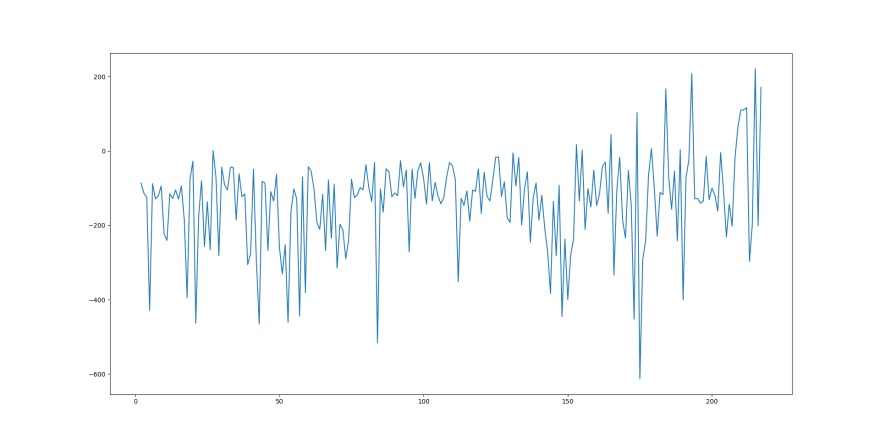
You might expect there to be a clearer trend showing the reward increasing over time. However, due to the exploration rate, this trend is distorted. As the episodes go on, the exploration rate decreases, so the expected trend of rewards increasing over time becomes slightly more apparent.

Here is how the agent performs at the end of the training process!

It could still do with a smoother landing, but I think this is a good performance nonetheless.

Maybe you could try this out yourself and tweak some of the training parameters and see what results they yield!

Original Link: https://dev.to/ashwinscode/teaching-an-ai-to-land-on-the-moon-5138

Share this article:

View Full Article

Dev To

An online community for sharing and discovering great ideas, having debates, and making friends

More About this Source Visit Dev To