
An Interest In:
Web News this Week
- April 2, 2024
- April 1, 2024
- March 31, 2024
- March 30, 2024
- March 29, 2024
- March 28, 2024
- March 27, 2024
Some of Our Sources
- Slashdot
- Team Treehouse
- Pearsonified
- Vandelay Design
- Creative Curio
- Fuel Your Creativity
- FanExtra - PSD
- Specky Boy
- Design Modo
- Willems Lab
Help Webnuz
Referal links:
Big O Notation: Time and Space Complexity
Efficiency is the word of the day. As humans we strive to be efficient in whatever we do, from moving around using Google Maps to having food delivered at our doorstep.
In computing, the computational complexity is the amount of resources required to run the algorithm. Resources in this case are the time and memory needed.
Time complexity is the amount of time taken by an algorithm as a function of the length of the input. Space complexity is the auxiliary memory taken by an algorithm to run as a function of the length of the input. Auxiliary memory is the lowest-cost, highest-space, and slowest-approach storage in a computer system.
Time and space are crucial since they determine how different computer programs are developed, designed and add value to the end user.
An ideal algorithm is one that takes less time and consumes
minimal space.
Algorithms just like humans optimizing tasks need to be executed optimally. Nothing is set in stone, most of the tradeoffs of time and space are in relation to the requirements. If the important thing of algorithm A is to run as fast as possible despite memory usage, we choose the most time efficient. While, if for the algorithm A, the vital thing is conserving space despite time, we select the most space efficient. Also, if we need to save both time and space we select one which uses an average amount of both time and space.
A good example of time and space complexity is as follows:
Example 1 to print one simple statement
import time# get the start timest = time.time()print("checking the time complexity example")# get the end timeet = time.time()# get the execution timeelapsed_time = et - stprint('Execution time:', elapsed_time, 'seconds')# output# checking the time complexity example# Execution time: 4.57763671875e-05 secondsExample 2 to print one simple statement 10 times
import time# get the start timest = time.time()for i in range(10): print("time complexity example")# get the end timeet = time.time()# get the execution timeelapsed_time = et - stprint('Execution time:', elapsed_time, 'seconds')# output# time complexity example# time complexity example# time complexity example# time complexity example# time complexity example# time complexity example# time complexity example# time complexity example# time complexity example# time complexity example# Execution time: 6.031990051269531e-05 secondsThe execution time differs for both since example one runs a simple statement(execution time of 4.57763671875e-05 seconds) while example two has a FOR Loop and the time taken is subject to the value of N, which in our case is 10 times(execution time of 6.031990051269531e-05 seconds).
The two examples above clearly illustrate that for algorithms that use statements execute once and require same amount of time. While statements that have conditions like Loops will increase depending on the number of times the Loop should run. For algorithms with combinations of Loops or nested Loops and single statements, time increases proportionately based on the number of times each and every statement should run.
Big O Notation
Big O Notation is used to describe the complexity of an algorithm using algebra terms. We use Big O to express running time of algorithms relative to its input, as the input size increases.
Types of Complexities
Constant time O(1)
An algorithm has constant time when it does not depend on the input size. Which means whether the input size increases or not, the runtime will always be the same.Linear time O(n)
An algorithm has linear time complexity when the run time increases with increase in the length of the input.Logarithmic time O (log n)
An algorithm has logarithmic time complexity when the size of input decreases in each step, which means that the input size is not the same as the operations being done. Operations increase as the input size increases. This is commonly seen in binary trees or binary search trees, where to search values you split the array into two, to ensure operation is not done on every element of the data.Quadratic time O (n^2)
An algorithm has quadratic time when the time increases non-linearly (n^2) with the length of the input. To exemplify nested Loops use this where one Loop has O(n), then finds another Loop which goes for O(n)*O(n) = O(n^2).
If say there are 'm' Loops defined, the order will be O(n ^ m). This is called polynomial time complexity functions.
 Order of growth for all time complexities
Differences in Time and Space Complexity
| Time | Space |
|---|---|
| Calculates the time taken | Estimates the memory required |
| Time is counted for each and every statement | Memory is counted for all outputs |
| Input data is the main determinant | The variable size is the main determinant |
| Vital for solution optimization | Essential for solution optimization |
Cheatsheets
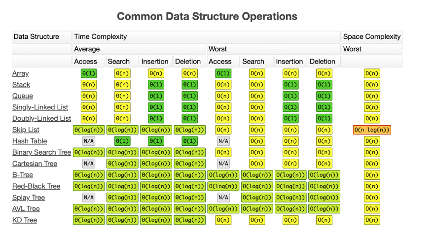 Common Data structure Space and Time Complexity Cheatsheet
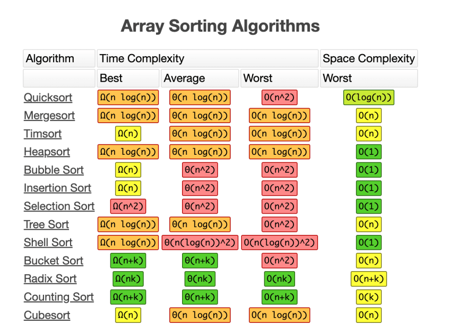 Array Sorting Algorithms Space and Time Complexity Cheatsheet
Conclusion
Through this article we have explored what time and space complexity and why we use Big O notation. Whether you are interviewing or learning this for the first time out of curiosity I hope this knowledge sticks with you.
Resources
Complexities
Guide to Complexity
Cheatsheet
Time Complexity
Complexity differences
Big O Notation
Original Link: https://dev.to/veldakiara/big-o-notation-time-and-space-complexity-14kk
Dev To
More About this Source Visit Dev To