Say hello to Big (O)h!

Oh or rather O, chosen by Bachmann to stand for Ordnung, meaning the Order of approximation.

"Wait, what is this guy saying?"

Helloooo and welcome back! Do not mind my curtain-raiser for this article for what we are going to be covering is super easy. It is known as The Big O notation.

According to wikipedia, the Big O notation is a mathematical notation that describes the limiting behavior of a function when the argument tends towards a particular value or infinity and characterizes functions according to their growth rates where different functions with the same growth rate may be represented using the same O notation.

Ooh oh! Not again.
In simple terms, (as used in Data Structures), the Big O notation is a way of comparing two sets of code, super simple, right?

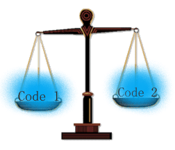
Assuming Code 1 and Code 2 accomplish exactly the same thing, how would you compare one to the other? Code 1 might be more readable while Code 2 can be more concise. Big O is a way of comparing Code 1 and Code 2 mathematically on their efficiency as they run.
Assuming too that you have a stopwatch, and we run Code 1 and start the stopwatch and the code runs for 15 seconds, then we reset the stopwatch and run Code 2 together with the stopwatch and it runs for 1 minute, based on this, we can say Code 1 is more efficient than Code 2. This is called Time Complexity.
The thing about Time Complexity that is interesting is that it is not measured in time. This is because if you took the same code and run it on a computer that runs twice as fast, it will complete twice as fast which does not make the code better but rather the computer is better. Time Complexity is therefore measured in the number of operations that it takes to complete something, a topic we will look deeper into with more examples in the course.

In addition to Time Complexity, we also measure Space Complexity. Despite Code 1 running super fast comparatively, it possibly might be taking a lot of memory space and maybe Code 2, despite taking more time in execution, may be taking less space in memory. If preserving memory space is your most important priority and you don't mind having some extra Time Complexity, maybe Code 2 is better.
It is therefore best to understand both concepts to be able to address the most important priority when given an "interview question" on either of the concepts either being a program that runs super fast or either one that conserves memory space.

When dealing with Time Complexity and Space Complexity, there are three greek letters one will interact with: (omega), (theta), and O (omicron).

• Assuming you have a list with seven items, and you are to build a for loop to iterate through it to find a specific number:

#Assuming we are looking for number '1', number '4' and number '7' in the list below:[1, 2, 3, 4, 5, 6, 7]

To get the number '1', we are going to find it in one operation, hence it's our best-case scenario but when we are looking for the number '7', we have to iterate through the entire list to find it, hence it's our worst-case scenario. If looking for the number '4', it's our average-case scenario.
When one is talking about the 'best-case scenario', that's (omega), while talking about the 'average-case scenario', that's (theta) and while talking about the worst-case scenario, that's O (omicron). Hence, technically when talking about Big O, we are talking mainly of the worst-case scenario.

To start with, we will mainly focus on the Time complexity.
We are gonna discuss different types of Big O notations as printed on my 'sweatshirt' below (Never Mind! haha):

Below are images with some characteristics we will discuss for each notation on their complexities:

Disclaimer: I have used Python code to explain each complexity.

• O(n)

This is one of the easiest Big O to explain. Let's use some code to explain this:

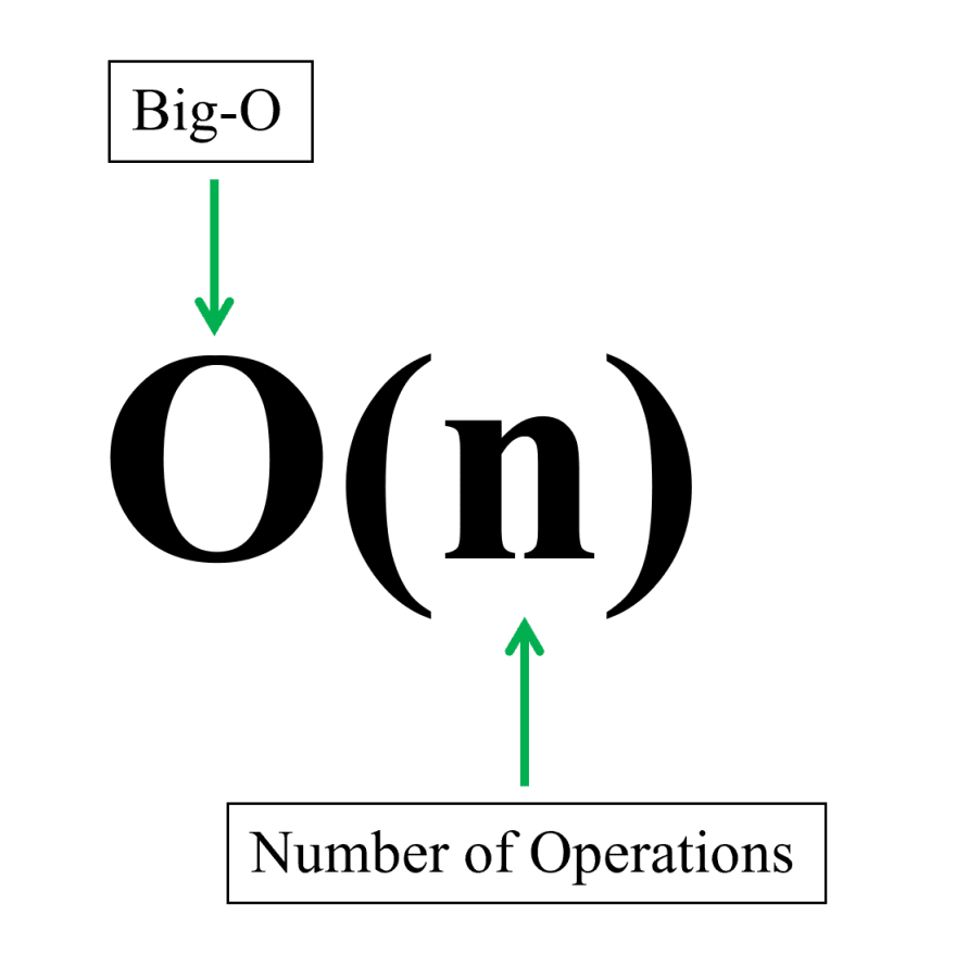
def print_items(n):    for i in range(n):        print(i)print_items(10)0123456789

The above print_items function is an example of something that is O(n). n stands for the number of operations. We passed in the function number 'n' and it ran n times\ 'n' operations.

Visualizing this on a graph:

   |                              *   |                    O(n) * T |                    * i |               * m |          * e |     *   |_*_ _ _ _ _ _ _ _ _ _ _ _ _ _ _ _ _                 input size

O(n) is always proportional hence it will always be a straight line.

• Drop Constants

There are a few ways in which we can simplify the Big O notation. The first one is known as the drop constant.
Using our previous example: print_items function, we are gonna add a second identical for loop:

def print_items(n):    for i in range(n):        print(i)    for j in range(n):        print(j)print_items(10)01234567890123456789

The above operation ran n + n times\ 2n number of operations which we write as O(2n) but we can simplify this by dropping the constant 2 and writing it as O(n). We can therefore drop all constants, eg. O(10n), O(100n), O(10000n) == O(n).

• O(n^2)

Adding a loop in another loop (nested for loop) using our previous example:

def print_items(n):    for i in range(n):       for j in range(n):          print(i, j)print_items(10)0 00 10 20 30 40 50 60 70 80 91 01 11 21 31 41 51 61 71 81 92 02 12 22 32 42 52 62 72 82 93 03 13 23 33 43 53 63 73 83 94 04 14 24 34 44 54 64 74 84 95 05 15 25 35 45 55 65 75 85 96 06 16 26 36 46 56 66 76 86 97 07 17 27 37 47 57 67 77 87 98 08 18 28 38 48 58 68 78 88 99 09 19 29 39 49 59 69 79 89 9

The above function runs n * n == n^2 hence we get the O(n^2). By adding an extra for loop and taking the function deeper (my apologies, the output will be a bit longer but will easily help you to understand how this works out):

def print_items(n):   for i in range(n):      for j in range(n):         for k in range(n):            print(i, j, k)print_items(10)0 0 00 0 10 0 20 0 30 0 40 0 50 0 60 0 70 0 80 0 90 1 00 1 10 1 20 1 30 1 40 1 50 1 60 1 70 1 80 1 90 2 00 2 10 2 20 2 30 2 40 2 50 2 60 2 70 2 80 2 90 3 00 3 10 3 20 3 30 3 40 3 50 3 60 3 70 3 80 3 90 4 00 4 10 4 20 4 30 4 40 4 50 4 60 4 70 4 80 4 90 5 00 5 10 5 20 5 30 5 40 5 50 5 60 5 70 5 80 5 90 6 00 6 10 6 20 6 30 6 40 6 50 6 60 6 70 6 80 6 90 7 00 7 10 7 20 7 30 7 40 7 50 7 60 7 70 7 80 7 90 8 00 8 10 8 20 8 30 8 40 8 50 8 60 8 70 8 80 8 90 9 00 9 10 9 20 9 30 9 40 9 50 9 60 9 70 9 80 9 91 0 01 0 11 0 21 0 31 0 41 0 51 0 61 0 71 0 81 0 91 1 01 1 11 1 21 1 31 1 41 1 51 1 61 1 71 1 81 1 91 2 01 2 11 2 21 2 31 2 41 2 51 2 61 2 71 2 81 2 91 3 01 3 11 3 21 3 31 3 41 3 51 3 61 3 71 3 81 3 91 4 01 4 11 4 21 4 31 4 41 4 51 4 61 4 71 4 81 4 91 5 01 5 11 5 21 5 31 5 41 5 51 5 61 5 71 5 81 5 91 6 01 6 11 6 21 6 31 6 41 6 51 6 61 6 71 6 81 6 91 7 01 7 11 7 21 7 31 7 41 7 51 7 61 7 71 7 81 7 91 8 01 8 11 8 21 8 31 8 41 8 51 8 61 8 71 8 81 8 91 9 01 9 11 9 21 9 31 9 41 9 51 9 61 9 71 9 81 9 92 0 02 0 12 0 22 0 32 0 42 0 52 0 62 0 72 0 82 0 92 1 02 1 12 1 22 1 32 1 42 1 52 1 62 1 72 1 82 1 92 2 02 2 12 2 22 2 32 2 42 2 52 2 62 2 72 2 82 2 92 3 02 3 12 3 22 3 32 3 42 3 52 3 62 3 72 3 82 3 92 4 02 4 12 4 22 4 32 4 42 4 52 4 62 4 72 4 82 4 92 5 02 5 12 5 22 5 32 5 42 5 52 5 62 5 72 5 82 5 92 6 02 6 12 6 22 6 32 6 42 6 52 6 62 6 72 6 82 6 92 7 02 7 12 7 22 7 32 7 42 7 52 7 62 7 72 7 82 7 92 8 02 8 12 8 22 8 32 8 42 8 52 8 62 8 72 8 82 8 92 9 02 9 12 9 22 9 32 9 42 9 52 9 62 9 72 9 82 9 93 0 03 0 13 0 23 0 33 0 43 0 53 0 63 0 73 0 83 0 93 1 03 1 13 1 23 1 33 1 43 1 53 1 63 1 73 1 83 1 93 2 03 2 13 2 23 2 33 2 43 2 53 2 63 2 73 2 83 2 93 3 03 3 13 3 23 3 33 3 43 3 53 3 63 3 73 3 83 3 93 4 03 4 13 4 23 4 33 4 43 4 53 4 63 4 73 4 83 4 93 5 03 5 13 5 23 5 33 5 43 5 53 5 63 5 73 5 83 5 93 6 03 6 13 6 23 6 33 6 43 6 53 6 63 6 73 6 83 6 93 7 03 7 13 7 23 7 33 7 43 7 53 7 63 7 73 7 83 7 93 8 03 8 13 8 23 8 33 8 43 8 53 8 63 8 73 8 83 8 93 9 03 9 13 9 23 9 33 9 43 9 53 9 63 9 73 9 83 9 94 0 04 0 14 0 24 0 34 0 44 0 54 0 64 0 74 0 84 0 94 1 04 1 14 1 24 1 34 1 44 1 54 1 64 1 74 1 84 1 94 2 04 2 14 2 24 2 34 2 44 2 54 2 64 2 74 2 84 2 94 3 04 3 14 3 24 3 34 3 44 3 54 3 64 3 74 3 84 3 94 4 04 4 14 4 24 4 34 4 44 4 54 4 64 4 74 4 84 4 94 5 04 5 14 5 24 5 34 5 44 5 54 5 64 5 74 5 84 5 94 6 04 6 14 6 24 6 34 6 44 6 54 6 64 6 74 6 84 6 94 7 04 7 14 7 24 7 34 7 44 7 54 7 64 7 74 7 84 7 94 8 04 8 14 8 24 8 34 8 44 8 54 8 64 8 74 8 84 8 94 9 04 9 14 9 24 9 34 9 44 9 54 9 64 9 74 9 84 9 95 0 05 0 15 0 25 0 35 0 45 0 55 0 65 0 75 0 85 0 95 1 05 1 15 1 25 1 35 1 45 1 55 1 65 1 75 1 85 1 95 2 05 2 15 2 25 2 35 2 45 2 55 2 65 2 75 2 85 2 95 3 05 3 15 3 25 3 35 3 45 3 55 3 65 3 75 3 85 3 95 4 05 4 15 4 25 4 35 4 45 4 55 4 65 4 75 4 85 4 95 5 05 5 15 5 25 5 35 5 45 5 55 5 65 5 75 5 85 5 95 6 05 6 15 6 25 6 35 6 45 6 55 6 65 6 75 6 85 6 95 7 05 7 15 7 25 7 35 7 45 7 55 7 65 7 75 7 85 7 95 8 05 8 15 8 25 8 35 8 45 8 55 8 65 8 75 8 85 8 95 9 05 9 15 9 25 9 35 9 45 9 55 9 65 9 75 9 85 9 96 0 06 0 16 0 26 0 36 0 46 0 56 0 66 0 76 0 86 0 96 1 06 1 16 1 26 1 36 1 46 1 56 1 66 1 76 1 86 1 96 2 06 2 16 2 26 2 36 2 46 2 56 2 66 2 76 2 86 2 96 3 06 3 16 3 26 3 36 3 46 3 56 3 66 3 76 3 86 3 96 4 06 4 16 4 26 4 36 4 46 4 56 4 66 4 76 4 86 4 96 5 06 5 16 5 26 5 36 5 46 5 56 5 66 5 76 5 86 5 96 6 06 6 16 6 26 6 36 6 46 6 56 6 66 6 76 6 86 6 96 7 06 7 16 7 26 7 36 7 46 7 56 7 66 7 76 7 86 7 96 8 06 8 16 8 26 8 36 8 46 8 56 8 66 8 76 8 86 8 96 9 06 9 16 9 26 9 36 9 46 9 56 9 66 9 76 9 86 9 97 0 07 0 17 0 27 0 37 0 47 0 57 0 67 0 77 0 87 0 97 1 07 1 17 1 27 1 37 1 47 1 57 1 67 1 77 1 87 1 97 2 07 2 17 2 27 2 37 2 47 2 57 2 67 2 77 2 87 2 97 3 07 3 17 3 27 3 37 3 47 3 57 3 67 3 77 3 87 3 97 4 07 4 17 4 27 4 37 4 47 4 57 4 67 4 77 4 87 4 97 5 07 5 17 5 27 5 37 5 47 5 57 5 67 5 77 5 87 5 97 6 07 6 17 6 27 6 37 6 47 6 57 6 67 6 77 6 87 6 97 7 07 7 17 7 27 7 37 7 47 7 57 7 67 7 77 7 87 7 97 8 07 8 17 8 27 8 37 8 47 8 57 8 67 8 77 8 87 8 97 9 07 9 17 9 27 9 37 9 47 9 57 9 67 9 77 9 87 9 98 0 08 0 18 0 28 0 38 0 48 0 58 0 68 0 78 0 88 0 98 1 08 1 18 1 28 1 38 1 48 1 58 1 68 1 78 1 88 1 98 2 08 2 18 2 28 2 38 2 48 2 58 2 68 2 78 2 88 2 98 3 08 3 18 3 28 3 38 3 48 3 58 3 68 3 78 3 88 3 98 4 08 4 18 4 28 4 38 4 48 4 58 4 68 4 78 4 88 4 98 5 08 5 18 5 28 5 38 5 48 5 58 5 68 5 78 5 88 5 98 6 08 6 18 6 28 6 38 6 48 6 58 6 68 6 78 6 88 6 98 7 08 7 18 7 28 7 38 7 48 7 58 7 68 7 78 7 88 7 98 8 08 8 18 8 28 8 38 8 48 8 58 8 68 8 78 8 88 8 98 9 08 9 18 9 28 9 38 9 48 9 58 9 68 9 78 9 88 9 99 0 09 0 19 0 29 0 39 0 49 0 59 0 69 0 79 0 89 0 99 1 09 1 19 1 29 1 39 1 49 1 59 1 69 1 79 1 89 1 99 2 09 2 19 2 29 2 39 2 49 2 59 2 69 2 79 2 89 2 99 3 09 3 19 3 29 3 39 3 49 3 59 3 69 3 79 3 89 3 99 4 09 4 19 4 29 4 39 4 49 4 59 4 69 4 79 4 89 4 99 5 09 5 19 5 29 5 39 5 49 5 59 5 69 5 79 5 89 5 99 6 09 6 19 6 29 6 39 6 49 6 59 6 69 6 79 6 89 6 99 7 09 7 19 7 29 7 39 7 49 7 59 7 69 7 79 7 89 7 99 8 09 8 19 8 29 8 39 8 49 8 59 8 69 8 79 8 89 8 99 9 09 9 19 9 29 9 39 9 49 9 59 9 69 9 79 9 89 9 9

The above function run n * n * n times hence it becomes O(n^3) but using drop constants to simplify this, it can also be written as O(n^2).

Notice that the first and the last elements in the output of the function(s) respectively are: O(n) - 0, 9 || O(n^2) - 00, 99 || O(n^3) - 000, 999.

Visualizing it on a graph:

   |          *                     |  O(n^2) *               T |        *           i |       *      m |      *   e |    *    |_*_ _ _ _ _ _ _ _ _ _ _ _ _ _ _ _ _                 input size

O(n^2) graph is steeper than the O(n) graph. This means that O(n^2) is a lot less efficient than O(n) from a Time Complexity standpoint.

   |          *                  *   |  O(n^2) *              *  T |        *          * i |       *      * O(n) m |      *   * e |    * *   |_*_ _ _ _ _ _ _ _ _ _ _ _ _ _ _ _ _                 input size

• Drop Non-Dominants

The second way to simplify the Big O notation is known as drop non-dominants.
Using the nested for loop example:

def print_items(n):   for i in range(n):      for j in range(n):         print(i, j)   for k in range(n):      print(k)print_items(10)0 00 10 20 30 40 50 60 70 80 91 01 11 21 31 41 51 61 71 81 92 02 12 22 32 42 52 62 72 82 93 03 13 23 33 43 53 63 73 83 94 04 14 24 34 44 54 64 74 84 95 05 15 25 35 45 55 65 75 85 96 06 16 26 36 46 56 66 76 86 97 07 17 27 37 47 57 67 77 87 98 08 18 28 38 48 58 68 78 88 99 09 19 29 39 49 59 69 79 89 90123456789

The above function ran twice. The first nested loop (i and j) ran O(n^2) while the second single loop (k) ran O(n). Hence the total number of the output is O(n^2) + O(n) which can also be written as O(n^2 + n).
The main thing of 'n' we are concerned about is "what happens when we start having 'n' as a very large number?" eg. when we have 'n' as 100, n^2 == 10000, hence as a percentage of the total number of operations, the stand-alone 'n' will still remain to be 100, which is a very small portion of the number of operations, hence it is insignificant. In the equation O(n^2 + n), 'n^2' is the dominant term while the stand-alone 'n' is the non-dominant, we drop the non-dominant and the notation remains to be O(n^2).

• O(1)

In comparison to other Big Os we have covered, as 'n' gets bigger, the number of operations increases, but with this Big O...:

def add_items(n):   return n + nadd_items(5)10

...there is always a single operation, and an increase to 'n' does not lead to an increase in the number of operations(remains constant). return n + n + n == O(2) == O(1).
O(1) is also called constant time. This is because as 'n' increases, the number of operations will remain constant.
Visualizing it on a graph:

   |                                 |                     T |                     i |                m |           e |              O(1)    |_*_*_*_*_*_*_*_*_*_*_*_*_*_*_*_*_ _                 input size

As 'n' increases, there is no increase in Time Complexity. This makes it the most efficient big(O). Anytime that you can make something O(1), it is optimal as you can make it.

   |          *                  *   |  O(n^2) *              *  T |        *          * i |       *      * O(n) m |      *   * e |    * *           O(1)   |_*_*_*_*_*_*_*_*_*_*_*_*_*_*_*_ _ _                 input size

• O(log n)

In demonstrating and explaining this, we will start with an example.
Assuming we have a list and looking for number '1' in the list:

[1, 2, 3, 4, 5, 6, 7, 8]

The numbers should be sorted.
What we are going to do is to find the most efficient way of finding the number '1' from the list.
We will first divide the list into half and check whether the number is either in the first half or the second half. We will take the half with the number and do away with the other half. We will continue with the process till we find the number.

[1, 2, 3, 4] [5, 6, 7, 8] --- 1 is in the first half[1, 2] [3, 4] --- 1 is in the first half[1] [2] --- 1 is in the first half1 --- We finally remain with the number

We then count how many steps we took to find the number:

1. [1, 2, 3, 4] [5, 6, 7, 8] --- 1 is in the first half2. [1, 2] [3, 4] --- 1 is in the first half3. [1] [2] --- 1 is in the first half

We took 3 steps to find the number from a total of 8 items(numbers).
2^3 = 8 == log2 8 = 3
8 -- Total items
3 -- Steps taken to arrive to the final number after dividing the number into halves
We can have an example like: log2 1,073,741,824 = 31 meaning that you can divide that number 31 times into halves to get to the final number despite which item you're looking for.
O(log n) is more efficient that O(n) but slightly less in efficiency than O(1).

• O(nlog n)

This is a Big(O) used with some sorting algorithms like merge sort and quick sort. This is not an efficient Big(O), however, this is the most efficient that you can make a sorting algorithm, sorting various types of data besides numbers.

Different terms for input is a Big(O) concept that interviewers like to as kind of a gotcha question.

An example is the function below with different parameters:

def print_items(a, b):    for i in range(a):        print(i)    for j in range(b):        print(j)

When covering O(n), we mentioned dropping constants and hence you might think that because this has two loops in the function, it can be equated to O(2n) == O(n) WHICH IS WRONG.
Being that the function has two parameters, a - 'n1' cannot be equivalent to b - 'n2' hence the Big(O) is O(a + b).
Similarly:

def print_items(a, b):    for i in range(a):       for j in range(b):          print(i, j) 

...the Big(O) is O(a * b).

Big(O) of Lists

Assuming we have a list my_list = [11, 2, 23, 7]:
If we want to append a number 17 at the end, (my_list.append(17)), there will be no re-indexing of the original numbers in the list.
Same case applies when we want to pop the number from the list, (my_list.pop()), no re-indexing of the items will occur. This therefore becomes a Big(O) of O(1).

However, when we want to pop a number at the index of 0, (my_list.pop(0)), or insert a number at index 0, (my_list.insert(0, 13)), re-indexing of all the items in the list occurs. This therefore becomes a Big(O) of O(n).

What about inserting items at the middle of the list? (my_list.insert(1, 'Hi'))
Re-indexing of the items at the right of the inserted item occurs. It being at the middle cannot be referred to as O(1/2 n). This is because Big(O) measures worst case and secondly '1/2' is a constant, hence we drop the constant. Therefore the Big(O) of inserting and popping items from the middle of the list is O(n).

• Looking for the item in a list

When looking for number 7 in the list my_list = [11, 3, 32, 7], we will iterate over the entire list till we find 7 in the list hence the Big(O) is O(n). But when we are looking for a number using an index from the list, (my_list[3]), we will find the number in the index without iterating, hence the Big(O) is O(1).

Wrapping Up

When we take n to be 100;
O(1) == 1
O(log n) == 7
O(n) == 100
O(n^2) == 10000

This means that O(n^2) compared to the other 3 is very inefficient. The spread becomes even bigger when 'n' becomes larger.

When we take n to be 1000;
O(1) == 1
O(log n) == 10
O(n) == 1000
O(n^2) == 1000000

• Terminologies used to refer to the Big(O)s:

O(1) - Constant
O(log n) - Divide and Conquer
O(n) - Proportional (will always be a straight line)
O(n^2) - Loop within a loop

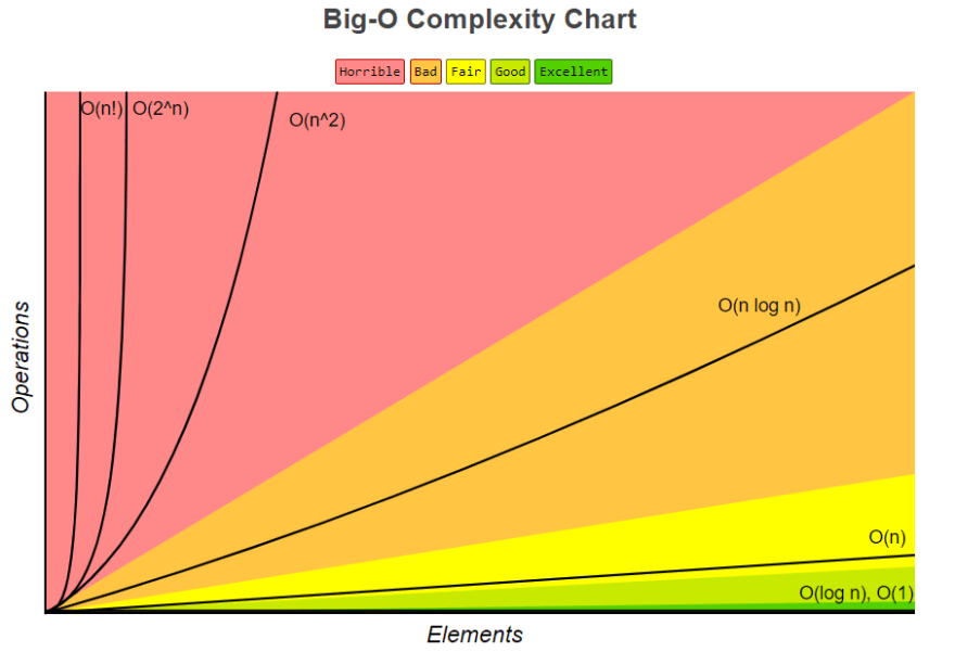
Summing it all up; We can now understand the chart below, that we had seen earlier in the course... however we didn't cover O(n!) and O(2^n) as they are not common and one has to intentionally write bad code to achieve.

Till Next time... Bye bye