CS50: Week 3, Sorting and Searching Algorithms

Since previous lectures, weve been learning about memory, how to store data in it, the types and sizes of data, among others things.

If we need to manage a large amount of data, it is convenient to use an array to store it, we already know how to do it, so this week David Malan teaches how to sort and search values in arrays explaining Searching Algorithms and Sorting Algorithms.

Big O and Big Omega

To understand the difference between distinct algorithms, we must first have a notion about Big O notation. In computer science, we can measure the efficiency of an algorithm in terms of memory consumption and running time. Big O notation is a special notation that measures running time, it tells you how fast an algorithm is, or how long an algorithm takes to run given some size of input. It doesnt measure running time in seconds or milliseconds, instead, it gives us an idea of how many operations an algorithm performs in relation to the input it receives.

Big O describes the upper bound of the number of operations, or how many steps an algorithm might take in the worst case until it finishes, while Big Omega notation (big ), in counterpart, describes the lower bound of the number of operations of an algorithm, or how few steps it might take in the best case.

The image above expresses the running time of three different ways of searching for a person in a phone book:

1. The red line represents searching on one page at a time starting from the beginning. It could take a lot of time find someone because the the searching becomes proportionally longer to complete as the phone book grows. If it takes 1 second to check 10 name, it will take 2 seconds to check 20 names, 3 seconds to check 30 names, 100 seconds to check 1000 names, and so on.

2. The yellow line represents searching on two pages at a time. It is double faster than the first option but still takes a lot of time to complete the search.

3. The green line represents the last and most efficient option, a divide and conquers approach. Open the phone book in the middle, if the target name is not there, then preserve the half where the name alphabetically must appear and discard the other half. Then repeat the process with the remaining half until the target is found. Its much faster than the other two options because the time required to find a name goes up linearly while the size of the phone book grows exponentially. So if it takes 1 second to check 10 names, it will take 2 seconds to check 100 names, 3 seconds to check 1000 names, and so on.
   
   
   In the chart above, if we zoomed out and changed the units on our axes, we would see the red and yellow lines end up very close together:

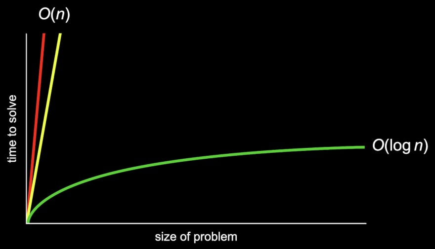
Since both the red and yellow lines end up being very similar as n becomes larger and larger, we can say they have the same time complexity. We would describe them both as having big O of n or on the order of n running time.

The green line, though, is fundamentally different in its shape, even as n becomes very large, so it takes big O of log n steps (later we will see why).

The most common running times are:

• O(n2) - Quadratic time
• O(n * log n) - Linearithmic time
• O(n) - Linear time
• O(log n) - Logarithmic time
• O(1) - Constant time

Linear Search

Is the simplest and intuitive method for finding an element within an array. The steps required to perform Linear Search would be:

1. Start from the leftmost element of the array.
2. Check if the target value matches the value stored in the array.
3. If matches, then the algorithm finishes successfully.
4. If it doesnt match, repeat step 2 with the next element of the array.
5. If the array finishes with no matches, then the target is not present in the array.

We might write the algorithm pseudocode as:

For each element from left to right    If number is at this position        Return trueReturn false

In the next example we search for the number 7:

list = [0, 2, 10, 4, 7, 9][0, 2, 10, 4, 7, 9] --> 0 is not equal to 7 ^[0, 2, 10, 4, 7, 9] --> 2 is not equal to 7    ^[0, 2, 10, 4, 7, 9] --> 10 is not equal to 7       ^[0, 2, 10, 4, 7, 9] --> 4 is not equal to 7           ^[0, 2, 10, 4, 7, 9] --> MATCH              ^The number 7 was found after 5 iterations

With n elements, well need to look at all n of them in the worst case (e.g. if we were searching for the number 9 in the example above), so the big O running time of this algorithm is linear O(n).

The lower bound, would be (1), since we might be lucky and find the number we are looking for at the first position of the array (e.g. if we were searching for the number 0 in the example above). (1) is also known as constant time, because a constant number of steps is required, no matter how big the problem is.

Linear Search is correct because it solves the searching problem, but it is not very efficient.

Just in case, this is my implementation of Linear Search in Python:

# Linear Searchdef linear_search(n, arr):    # Use the in operator to check if the target value     # is on the list    if n in arr:        return True    return Falseif __name__ == '__main__':    array = [53,9,6,23,8,5,4,1,88]    # Ask the user for a target value    number = int(input('Que nmero buscas?: '))    result = linear_search(number, array)    if result:        print('El nmero existe.')    else:        print('El nmero no existe.')

Binary Search

This method uses an approach called divide and conquer, where we divide the problem in half on each step. This algorithm works only on sorted arrays. The steps required to perform Linear Search would be:

1. Get an element from the middle of the array.
2. If the element matches the target value, then the algorithm finishes successfully.
3. If the target value is smaller than the middle element, narrow the array to the left half.
4. If the target value is greater than the middle element, narrow the array to the right half.
5. Repeat from step 1 with the narrowed array.
6. If the array is empty, then the target is not present in the array.

We might write the algorithm pseudocode as:

If array is empty    Return falseIf number is at the middle position    Return trueElse if number < number at the middle position    Search left halfElse if number > number at the middle position    Search right half

In the next example we search for the number 6:

list = [0, 1, 2, 3, 4, 5, 6][0, 1, 2, 3, 4, 5, 6] --> 3 is the middle element. 6 is higher so we search on the right half          ^[4, 5, 6] --> 5 is the middle element. 6 is higher so we search on the right half    ^[6] --> MATCH ^The number 6 was found after 3 iterations

The upper bound for binary search is O(log n), known as logarithmic time. When an algorithm has O(log n) running time, it means that as the input size grows, the number of operations grows very slowly. Since in Binary Search were discarding the half of the elements on every step, we can say that n (the size of the problem) is reduced exponentially, while the time required to find the target goes up linearly.

The best case scenario for this algorithm is to find the target exactly in the middle, in the first iteration, which means that the Big Omega running time is in the order of (1).

Even though binary search might be much faster than linear search, it requires our array to be sorted first. If were planning to search our data many times, it might be worth taking the time to sort it first, so we can use binary search.

To understand in-depth how Binary Search works we must know first what recursion is. If you look at the pseudocode again note that we're using the same search algorithm for the left and right half. That is recursion, the ability for a function to call itself.

This seems like a cyclical process that will never end, but were actually changing the input to the function and dividing the problem in half each time, stopping once there are no more elements left. When the function runs over elements, that is the condition, also known as base case, which tells the recursive function to stop, so it doesnt call itself over and over forever.


Here is my implementation of Binary Search written in Python:

# Binary Searchdef binary_search(n, arr, l):    # Base Case    # If there's only 1 element then check explcitly if matches the target value    if l == 1:        return True if arr[0] == n else False    # Calculate the middle of the list    mid = l // 2    # Check if the middle element matches the target    if arr[mid] == n:        return True    else:        # If the target is smaller, repeat the search on the left half         # otherwise, look in the right half.        if n < arr[mid]:            return binary_search(n, arr[:mid], len(arr[:mid]))        else:            return binary_search(n, arr[mid:], len(arr[mid:]))if __name__ == '__main__':    array = [53,9,6,23,8,5,4,1,88]    long = len(array)    # Ask the user for a target value    number = int(input('Que nmero buscas?: '))    # Sort the array with sorted() function since Binary Search works with sorted lists    result = binary_search(number, sorted(array), long)    if result:        print('El nmero existe.')    else:        print('El nmero no existe.')

Selection Sort

Selection Sort works by sorting arrays from left to right. The steps required to sort a list with this algorithm would be:

1. Start from the leftmost element of the array
2. Traverse the array to find the smallest element
3. After traversing the array, swap the smallest element with the value on the first position of the array
4. Repeat from step 2, now starting from the second element, and swap the smallest value with the value on the second position of the array. Continue repeating with the 3rd, 4td, and so on, until the array is sorted.

Because computers can only look at one number at a time, we must iterate over the entire array each time to find the smallest value, without taking into account already sorted elements.

We might write the algorithm pseudocode as:

For i from 0 to n1    Find smallest number between numbers[i] and numbers[n-1]    Swap smallest number with numbers[i]

In the next example we sort the next list:

list = [3, 6, 5, 7, 8, 2][3, 6, 5, 7, 8, 2] --> 2 is the smallest element                ^[2, 6, 5, 7, 8, 3] --> Swap it with the element on the first position ^              ^[2, 6, 5, 7, 8, 3] --> Now 3 is the smallest, since 2 is already sorted                ^[2, 3, 5, 7, 8, 6] --> Swap it with the element in the second position    ^           ^[2, 3, 5, 7, 8, 6] --> Now 5 is the smallest number. No swap needed because is already sorted       ^[2, 3, 5, 7, 8, 6] --> Repeat the process                ^[2, 3, 5, 6, 8, 7]          ^     ^[2, 3, 5, 6, 8, 7]                ^[2, 3, 5, 6, 7, 8]             ^  ^After 5 iterations the  array is sorted

We can say that the algorithm has an upper bound for running time of O(n2), because we will be iterating the array over and over, searching for the smallest number.

In the best case, where the list is already sorted, our selection sort algorithm will still look at all the numbers and repeat the loop, so it has a lower bound for running time of (n2).

Here is my implementation of Selection Sort written in Python:

# Selection Sortdef selection_sort(arr, l):    # If the list has just one item then it's already sorted    if l == 1:        return arr    # Loop over the entire list    for i in range(l):        lowest_index = None        # Loop over each element to find the smallest one        for j in range(i, l):            if lowest_index is None or arr[j] < arr[lowest_index]:                # Save the index of the smallest element                lowest_index = j        # Swap elements        # It's possible to swap elements like this in Python,        # avoiding the use of a temporary variable        (arr[i], arr[lowest_index]) = (arr[lowest_index], arr[i])    return arrif __name__ == '__main__':    array = [53,9,6,23,8,5,4,1,88]    long = len(array)    print(selection_sort(array, long))

Bubble Sort

This algorithm sorts elements from right to left using comparison and swapping elements. We compare contiguous pairs of elements and swapping both if the smaller is on the right, and repeating the entire loop until no swaps were needed anymore.

We could describe its functionality as follows:

1. Look at the first element of the array, which will be the current value.
2. Compare the current value with the next element in the array.
3. If the next element is smaller, swap both values. Save in a variable that a swap was performed.
4. Move to the next element of the array and make it the current value.
5. Repeat from step 2 until the last number in the list has been reached.
6. If any values were swapped, repeat again from step 1, without taking into account the last element of the array, which will be already sorted.
7. If the end of the list is reached without any swaps being made, then the list is sorted.

The pseudocode for bubble sort might look like:

Repeat n-1 times    For i from 0 to n2        If numbers[i] and numbers[i+1] out of order            Swap them    If no swaps        Quit

We are going to sort the same list we sorted with Selection Sort to see the differences:

list = [3, 6, 2, 7, 5][3, 6, 2, 7, 5] --> compare 3 and 6, they're sorted ^  ^[3, 6, 2, 7, 5] --> compare 6 and 2, swap them    ^  ^[3, 2, 6, 7, 5] --> compare 6 and 7, they're sorted       ^  ^[3, 2, 6, 7, 5] --> compare 7 and 5, swap them          ^  ^// Start from the beginning again[3, 2, 6, 5, 7] --> compare 3 and 2, swap them ^  ^[2, 3, 6, 5, 7] --> compare 3 and 6, they're sorted    ^  ^[2, 3, 6, 5, 7] --> compare 6 and 5, swap them       ^  ^// We don't compare 7 because is already sorted. At this point// we know that the array is sorted, but still we need to loop // through the array one more time to check that no more swaps // are needed[2, 3, 5, 6, 7] --> compare 2 and 3, they're sorted ^  ^[2, 3, 5, 6, 7] --> compare 3 and 5, they're sorted    ^  ^// At this point the algorithm finishes because there were no// swaps, and as in the previous iteration, we don't need to// compare the number 6 because is already sorted.After 3 iterations the array is sorted

We can say that bubble sort has an upper bound for running time of O(n2), because as with Selection Sort, we must iterate over the array once and once, but the difference is that the lower bound would be (n), because if the array is sorted just a single iteration over the array is needed to check that there were no swaps.


Here is my implementation of Bubble Sort written in Python:

# Bubble Sortdef bubble_sort(arr, l):    # If the list has just one item then it's already sorted     if l == 1:        return arr    # Loop over the entire list    for i in range(1, l):        # Swaps counter        swaps = 0        # Loop over the list to compare pairs of adjacent elements        for j in range(l-i):            if arr[j] > arr[j+1]:                # Swap elements                (arr[j], arr[j+1]) = (arr[j+1], arr[j])                swaps += 1        # If there were no swaps, then the array is sorted        if swaps == 0:            return arrif __name__ == '__main__':    array = [53,9,6,23,8,5,4,1,88]    long = len(array)    print(bubble_sort(array, long))

Merge Sort

This algorithm also makes use of the divide and conquer approach, and the recursion technique, just like Binary Search does. It divides the input array into two halves, calls itself for the two halves until it get an array containing one element (which is considered sorted), and then it repeatedly merges each sorted halves.

We could describe the algorithm with the following steps

1. Find the middle of the array.
2. Divide the array from the middle.
3. Call Merge Sort for the left half of the array.
4. Call Merge Sort for the right half of the array.
5. Merge the two sorted halves into a single sorted array

As were using recursion, each call to Merge Sort will perform all the steps (from 1 to 5) for the sublist it receives. The base case, when Merge Sort stops calling itself, is when it receives an array with just one element since an array of one element is already sorted.

The pseudocode for bubble sort might look like:

If only one number  QuitElse    Sort left half of number    Sort right half of number    Merge sorted halves

It could be difficult to understand the algorithm just by words, so an example could help to show how Merge Sort works.

In the example below, the red arrows represent each call to Merge Sort, which divides the array it receives into two sublists; and the green arrows represent the merging operation.

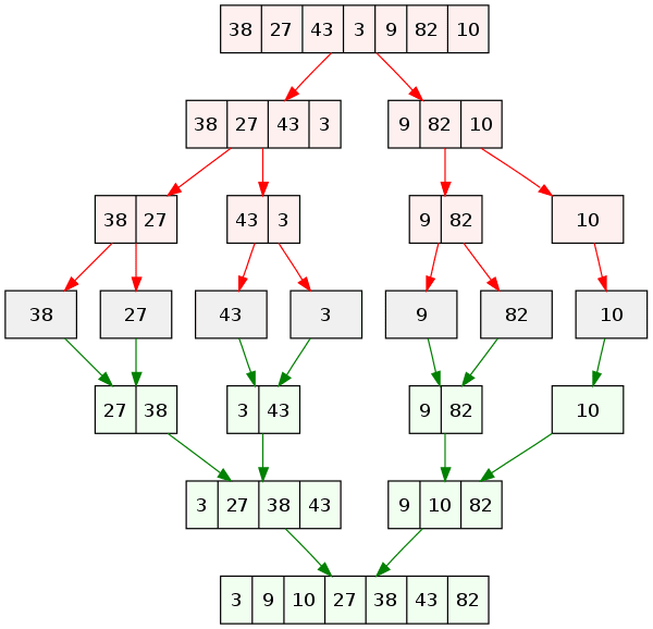
The strategy is to sort each half, and then merge them. The merging operation works as follows:

Compare the leftmost element of both sublists and move the smallest value to a new array. Repeat the process until both sublists are merged into one array.

If we want to merge the last two sublists of the example above, the steps are the following:

// Compare the first element of each sublist and copy the smallest value // to a new array[3, 27, 38, 43]  [9, 10, 82]  =>  [3] ^                ^[27, 38, 43]     [9, 10, 82]  =>  [3, 9] ^                ^[27, 38, 43]     [10, 82]     =>  [3, 9, 10] ^                ^[27, 38, 43]     [82]         =>  [3, 9, 10, 27] ^                ^[38, 43]         [82]         =>  [3, 9, 10, 27, 38] ^                ^[43]             [82]         =>  [3, 9, 10, 27, 38, 43] ^                ^[]               [82]         =>  [3, 9, 10, 27, 38, 43, 82]                  ^

The base case for our recursive function will be a list containing just one element, as I said before, a list of one element is considered sorted.

The time complexity of Merge Sort is O(n Log n), as the algorithm always divides the array into two halves, which have a complexity of O(log n); and the merge operation takes linear time, or O(n), since we only need to look at each element once.

The lower bound of our merge sort is still (n log n), since we have to do all the work even if the list is sorted.


Here is my implementation of Merge Sort written in Python:

# Merge Sortdef merge_sort(arr, l):    # Base case    if l == 1:        return arr    # Calculate the middle of the list    mid = l // 2    # Call merge sort for left and right halves    left = merge_sort(arr[:mid], len(arr[:mid]))    right = merge_sort(arr[mid:], len(arr[mid:]))    # Calculate how many elements must be merged    merge_q = len(left) + len(right)    # Empty list were the sublists will be merged into    sorted_array = []    for i in range(merge_q):        # If both sublists have elements to be sorted        if len(left) > 0 and len(right) > 0:            # Append smallest value to the sorted list            if left[0] >= right[0]:                sorted_array.append(right[0])                del(right[0])            else:                sorted_array.append(left[0])                del(left[0])        # If right half is empty append left half to the sorted list        elif len(left) > 0:            sorted_array.append(left[0])            del(left[0])        # If left half is empty append right half to the sorted list        else:            sorted_array.append(right[0])            del(right[0])    return sorted_arrayif __name__ == '__main__':    array = [53,9,6,23,8,5,4,1,88]    length = len(array)    print(merge_sort(array, length))

I hope you found interesting searching and sorting algorithms, as I found it when taking the class. There are other algorithms, but this is a good first approach to this topic.

The next lecture is about memory: addresses, pointers, allocation, and other concepts to continue learning how computer software works.

I hope you find interesting what Im sharing about my learning path. If youre taking CS50 also, leave me your opinion about it.

See you soon!

Thanks for reading. If you are interested in knowing more about me, you can give me a follow or contact me on Instagram, Twitter, or LinkedIn .