How we scaled ingestion to one million rows per second

This post was written by Niklas Schmidtmer and originally published at crate.io

One of CrateDBs key strengths is scalability. With a truly distributed architecture, CrateDB serves high ingest loads while maintaining sub-second reading performance in many scenarios. In this article, we want to explore the process of scaling ingestion throughput. While scaling, one can meet a number of challenges - which is why we set ourselves the goal of scaling to an ingest throughput of 1,000,000 rows/s. As CrateDB indexes all columns by default, we understand ingestion as the process of inserting data from a client into CrateDB, as well as indexing.

But this should not become yet another artificial benchmark, purely optimized at showing off numbers. Instead, we went with a representative use case and will discuss the challenges we met on the way to reaching the 1,000,000 rows/s throughout.

Table of content

• The aim
• The strategy
  • The ingest process
• The benchmark process
• The data model
• The tools
• The infrastructure
• The results
  • Single-node
  • Scaling out
• The conclusion
• The learnings

The aim

Besides the number of 1,000,000 rows/s, we set ourselves additional goals, to remain as close as possible to real-world applications:

• Representativeness: The data model must be representative, including numerical as well as textual columns in a non-trivial structure.
• Reproducibility: The provisioning of all involved infrastructure components should be highly automated and must be easily reproducible.
• Realism: No shortcuts shall be taken in the sole interest of increasing throughput, such as disabling CrateDBs indexing.
• Sustainability: The target throughput must be reached as an average value over a timespan of at least five minutes.

The strategy

The overall strategy to reach the throughput of 1,000,000 rows/s is relatively straightforward:

1. Start a single-node cluster and find the ingest parameter values that yield the best performance
2. Add additional nodes one by one until reaching the target throughput

The single-node cluster will set the baseline throughput for one node. At a first glance, it could be assumed that the number of required nodes to reach the target throughout can be calculated as 1,000,000 / baseline throughput.

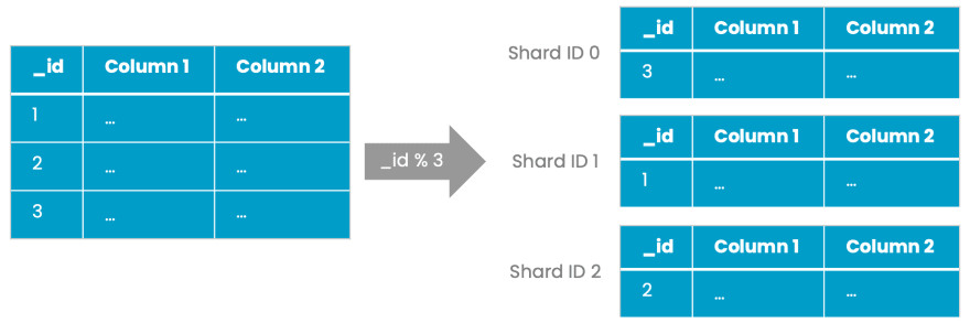
Lets revisit at this point CrateDBs architecture. In CrateDB, a table is broken down into shards, and shards are distributed equally across the nodes. The nodes form a fully meshed network.

The ingest process

With that cluster architecture in mind, lets break down the processing of a single INSERT statement:

1. A client sends a batched INSERT statement to any of the nodes. We call the selected node the query handler node.
   
   We will later be utilizing a load balancer with a round-robin algorithm to ensure that the query handling load is distributed equally across the cluster.

2. The query handler node parses the INSERT statement and assigns each row a unique ID (_id). Based on this ID and certain shard metadata, the query handler node assigns each row the corresponding target shard. From here, two scenarios can apply:

   1. The target shard is located on the query handler node. Rows get added to the shard locally.
   2. The target shard is located on a different node. Rows are serialized on the query handler node, transmitted over the network to the target node, deserialized, and finally written to the target shard.

For additional information on custom shard allocation, please see the CREATE TABLE documentation.

Scenario 2.a is best from a performance perspective, but as each node holds an equal number of shards (number of total shards / number of nodes), scenario 2.b will be the more frequent one. Therefore, we have to expect a certain overhead factor when scaling and throughput will be lower than baseline throughput * number nodes.

The benchmark process

Before running any benchmarks, the core question is: How to identify that a node/cluster has reached its optimal throughput?

The first good candidate to look at is CPU usage. CPU cycles are required for query handling (parsing, planning, executing queries) as well as for the actual indexing of data. A CPU usage in the range of consistently > 90% is a good first indicator that the cluster is well utilized and busy.

But looking at CPU usage alone can be misleading, as there is a fine line between well utilizing and overloading the cluster.

In CrateDB, each node has a number of thread pools for different operations, such as reading and writing data. A thread pool has a fixed number of threads that process operations. If no free thread is available, the request for a thread is rejected and the operation gets queued.

To reach the best possible throughput, we aim to keep threads fully utilized and have the queue of INSERT queries filled sufficiently. Threads should never be idle. However, we also don't want to overload the queue so that queueing time negatively impacts the throughput.

The state of each nodes' thread pools can be inspected via the system table sys.nodes. The below query sums up all rejected operations across all thread pools and nodes. Note that this metric isnt historized, so the number represents the total of rejected operations since the nodes' last restart.

SELECT SUM(pools['rejected'])FROM (  SELECT UNNEST(thread_pools) AS pools  FROM sys.nodes) x;

In our benchmarks, we will increase concurrent INSERT queries up to a maximum where no significant amount of rejections appear.

For a more permanent monitoring of rejected operations and several more metrics, take a look at CrateDBs JMX monitoring as well as CrateDB and Prometheus for long-term metrics storage.

The data model

On the CrateDB side, the data model consists of a single table that stores CPU usage statistics from Unix-based operating systems. The data model was adopted from Timescales Time Series Benchmark Suite.

The tags column is a dynamic object which gets provided as a JSON document during ingest. This JSON document described the host on which the CPU metrics were captured.

One row consists of 10 numeric metrics, each modeled as top-level columns:

CREATE TABLE IF NOT EXISTS doc.cpu (  "tags" OBJECT(DYNAMIC) AS (    "arch" TEXT,    "datacenter" TEXT,    "hostname" TEXT,    "os" TEXT,    "rack" TEXT,    "region" TEXT,    "service" TEXT,    "service_environment" TEXT,    "service_version" TEXT,    "team" TEXT  ),  "ts" TIMESTAMP WITH TIME ZONE,  "usage_user" INTEGER,  "usage_system" INTEGER,  "usage_idle" INTEGER,  "usage_nice" INTEGER,  "usage_iowait" INTEGER,  "usage_irq" INTEGER,  "usage_softirq" INTEGER,  "usage_steal" INTEGER,  "usage_guest" INTEGER,  "usage_guest_nice" INTEGER) CLUSTERED INTO <number of shards> SHARDSWITH (number_of_replicas = 0);

The number of shards will be determined later as part of the benchmarks. Replications (redundant data storage) are disabled so that we can measure the pure ingest performance.

All other table settings remain at their default values, which also means that all columns will get indexed.

The tools

To provision the infrastructure that our benchmark is running on, as well as generating the INSERT statements, we make use of two tools:

• crate-terraform: Terraform scripts to easily start CrateDB clusters in the cloud. For a certain set of variable values, it spins up a CrateDB cluster in a reproducible way (including a load balancer). It also allows configuring certain performance-critical properties, such as disk throughput. Going with Terraform guarantees that the setup will be easy to reproduce. We will run all infrastructure on the AWS cloud.

• nodeIngestBench: The client tool generating batched INSERT statements. Implemented in Node.js, it provides the needed high concurrency with a pool of workers that run as separate child processes.

The infrastructure

For CrateDB nodes, we chose m6g.4xlarge instances. Based on AWS' Graviton 2 ARM architecture, they provide powerful resources at a comparably low cost. With 16 CPU cores and 64 GB RAM, we try to get a high base throughput for a single node, and therefore keep the number of nodes low.

Each node has a separate disk containing CrateDBs data directory, which we provision with 400 MiB/s throughput and 5000 IOPS, so that disks will not become a bottleneck.

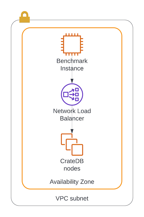
Additionally, we spin up another EC2 instance that will run the Node.js ingest tool. The benchmark instance is an m6g.8xlarge instance. We do not actually require the 32 CPU cores and 128 GB RAM that it provides, but it is the smallest available instance type with a guaranteed network throughput of 12 Gbps.

To keep latency between the CrateDB cluster and the benchmark instance as low as possible, all of them are placed in the same subnet. We also configure the load balancer to be an internal one, so that all traffic remains within the subnet.

Below is the complete Terraform configuration. Please see crate-terraform/aws for details on how to apply a Terraform configuration.

module "cratedb-cluster" {  source = "[email protected]:crate/crate-terraform.git//aws"  region = "eu-west-1"  vpc_id             = "vpc-..."  subnet_ids         = ["subnet-..."]  availability_zones = ["eu-west-1b"]  ssh_keypair = "cratedb_terraform"  ssh_access  = true  instance_type         = "m6g.4xlarge"  instance_architecture = "arm64"  # The size of the disk storing CrateDB's data directory  disk_size_gb = 100  disk_iops       = 5000  disk_throughput = 400 # MiB/s  # CrateDB-specific configuration  crate = {    # Java Heap size in GB available to CrateDB    heap_size_gb = 50    cluster_name = "crate-cluster"    # The number of nodes the cluster will consist of    cluster_size = 1 # increase to scale the cluster    ssl_enable = true  }  enable_utility_vm      = true  load_balancer_internal = true  cratedb_tar_download_url = "https://cdn.crate.io/downloads/releases/cratedb/aarch64_linux/crate-4.7.0.tar.gz"  utility_vm = {    instance_type         = "m6g.8xlarge"    instance_architecture = "arm64"    disk_size_gb          = 50  }}output "cratedb" {  value     = module.cratedb-cluster  sensitive = true}

The results

Each benchmark run is represented by a corresponding call of our nodeIngestBench client tool with the following call:

node appCluster.js \  --batchsize 15000 \  --shards <number of shards> \  --processes <processes> \  --max_rows 30000000 \  --concurrent_requests <concurrent requests>

Lets break down the meaning of each parameter:

• batchsize: The number of rows that are passed in a single INSERT statement. A relatively high value of 15.000 rows keeps the query handling overhead low.

• shards: The number of shards the table will be split into. Each shard can be written independently, so we aim for a number that allows for enough concurrency. On adding a new node, we will increase the number of shards. Shards are automatically distributed equally across the cluster. For a real-world table setup, please also consider our Sharding and Partitioning Guide for Time Series Data.

• processes: The main nodeprocess will start this number of child processes (workers) that generate INSERT statements in parallel.

• max_rows: The maximum number of rows that each child process will generate. It can be used to control the overall runtime of the tool. We will lower it slightly when scaling to keep the runtime at around five minutes.

• concurrent_requests: The number of INSERT statements that each child process will run concurrently as asynchronous operations.

Single-node

We start simple with a single node deployment to determine the throughput baseline. As we have 16 CPU cores, we chose the same amount of shards. A single process with a concurrency of 16 queries shows a throughput of 171,242 rows/s.

Scaling out

We scale horizontally, by adding one additional node at a time. With each node, we also add another ingest client process to increase concurrency.

However, as indicated before, with every additional node, the node-to-node traffic also increases. Since this has a negative impact on the cluster-wide throughput, we cannot scale the ingest load in a strictly linear way. Instead, we observe the rejected thread pool count after each scaling and decrease the concurrent_requests parameter by one if needed.

Below are the full results, which also include all required information to reproduce the benchmark run on your own:

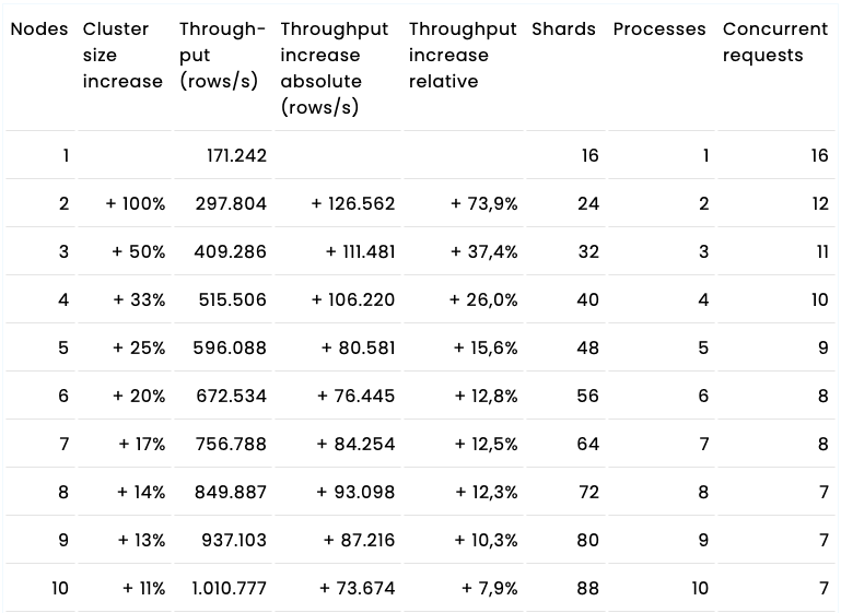
We reach the target throughput of 1,010,777 rows/s with a 10 node cluster. As each rows contains 10 metrics, it equals a throughput of 10,107,774 metrics/s.

The max_rows parameter was reduced from 30 million rows per child process to 28 million rows for the 10 node cluster to remain within a runtime of five minutes. Overall, this leads to a table cardinality of 280 million rows, consuming 48 GiB of disk space (including indexes, after running OPTIMIZE TABLE).

Assuming each node in the 10-node cluster contributed equally to the overall throughput, this means a per-node throughput of 101,078 rows/s. It can be seen that the per-node throughput continuously decreases while scaling:

The conclusion

Our ingest scenario replicated a use case of 10 concurrently ingesting clients. Each sent seven queries in parallel and generated 28 million rows (280 million metrics) that were ingested at a (calculative) rate of slightly above one million rows per second.

With every additional node, we simulated the addition of another client process and saw a linear increase in throughput. With increasing cluster size, the throughput per node slightly decreased. This can be explained by the increasing distribution of data and the greater impact of node-to-node network traffic. Once a certain cluster size is reached, the impact of that effect becomes less.

As a consequence, plotting the measured throughput in comparison to the projected throughput (excluding any overhead) of measured throughput before scaling * (1 + cluster size increase), shows that both lines clearly diverge from each other:

To take the node-to-node communication overhead into consideration, we reduce the projected throughput by 25% on each scaling (measured throughput before scaling * (1 + (0,75 * cluster size increase))):

Measured and expected throughput now match very closely, indicating that on each scaling, 25% of the cluster size increase is taken up by the node-to-node communication.

Despite the overhead, our findings still clearly show that scaling a CrateDB cluster is an adequate measure to increase ingest throughput without having to sacrifice indexing.

The learnings

We want to wrap up these results with a summary of the learnings we made throughout this process. They can serve as a checklist for your CrateDB ingest tuning as well:

• Disk performance: The disks storing CrateDBs data directory must have enough throughput. SSD drives are a must-have for good performance, peak-throughout can easily reach rates of > 200 MiB/s. Monitor your disk throughput closely and be aware of hardware restrictions.

• Network performance: The throughput and latency of your network become relevant at high ingest rates. We saw outgoing network throughput of around 10 GiB/s from the benchmark instance towards the CrateDB cluster. As node-to-node traffic increases while scaling, ensure it also provides enough performance. When running in the cloud, certain instance types have restricted network performance. When working with a mixture of public and private IP addresses/hosts, ensure to consistently use the private ones to prevent traffic needlessly being routed through the slower public internet.

• Client-side performance: Especially when generating artificial benchmark data from a single tool, understand its concurrency limitations. In our case with Node.js, we initially generated asynchronous requests in a single process, but still didnt get the maximum out of it. In Node.js, each process is still limited by a thread pool for asynchronous events, so only a multi-process approach was able to overcome this barrier. Always batch your INSERT statements, dont use single statements.

• Modern hardware: Use a modern hardware architecture. More recent CPU architectures have a performance advantage over older ones. A 16 CPU cores desktop machine will not be able to match the speed of a 16 CPU cores server architecture of the latest generation.