
An Interest In:
Web News this Week
- April 20, 2024
- April 19, 2024
- April 18, 2024
- April 17, 2024
- April 16, 2024
- April 15, 2024
- April 14, 2024
Some of Our Sources
- Engadget
- Six Revisions
- Abduzeedo
- Vandelay Design
- Line 25
- Stylized Web
- Design Modo
- Android Dissected
- Willems Lab
- Daily Now
Help Webnuz
Referal links:
A Gentle Introduction to Reinforcement Learning
A gentle introduction to Reinforcement Learning
In 2016, AplhaGo, a program developed for playing the game of Go, made headlines when it beat the world champion Go player in a five-game match. It was a remarkable feat because the number of possible legal moves in Go are of the order of 2.1 10170. To put this in context, this number is far, far greater than the number of atoms in the observable universe, which are of the order of 1080. Such a high number of possibilities make it almost impossible to create a program that can play effectively using brute-force or somewhat optimized search algorithms.
A part of the secret sauce of AlphaGO was the usage of Reinforcement Learning to improve its understanding of the game by playing against itself. Since then, the field of Reinforcement Learning has seen increased interest, and much more efficient programs have been developed to play various games at a pro-human efficiency. Although you would find Reinforcement Learning discussed in the context of Games and Puzzles in most places (including this post), the applications of Reinforcement Learning are much more expansive. The objective of this tutorial is to give you a gentle introduction to the world of Reinforcement Learning.
First things first! This post was written in collaboration with Alexey Vinel (Professor, Halmstead University). Some ideas and visuals are borrowed from my previous post on Q-learning written for Learndatasci. Unlike most posts you'll find on Reinforcement learning, we try to explore Reinforcement Learning here with an angle of multiple agents. So this makes it slightly more complicated and interesting at the same time. While this will be a good resource to develop intuitive understanding of Reinforcement Learning (Reinforcement Q-learning to be specific), it is highly recommended to visit the theoretical parts (some links shared in the appendix), if you're willing to explore Reinforcement Learning beyond this post.
I had to fork openAIs gym library to implement a custom environment. The code can be found on this github repository. If you'd like to explore an interactive version, you can check out this google colab notebook. We use Python to implement the algorithms, if you're not familiar with Python you can simply pretend that those snippets don't exist and read through the textual part (including code comments). Alright, time to get started
What is Reinforcement Learning?
Reinforcement learning is a paradigm of Machine Learning where learning happens through the feedback gained by an agent's interaction with its environment. This is also one of the key differentiators of Reinforcement Learning with the other two paradigms of Machine learning (Supervised learning and Unsupervised learning). Supervised learning algorithms require fully labelled-training-data, and Unsupervised learning algorithms need no labels. On the other hand, Reinforcement learning algorithms utilize feedback from the environment they're operating in to get better at the tasks they're being trained to perform. So we can say that Reinforcement Learning lies somewhere in the middle of the spectrum.
It is inevitable to talk about Reinforcement Learning with clarity without using some technical terms like "agent", "action", "state", "reward", and "environment". So let's try to gain a high-level understanding of Reinforcement Learning and these terms through an analogy,
Understanding Reinforcement learning through Birbing
Let's watch the first few seconds of this video first,
Pretty cool, isn't it?
And now think about how did someone manage to teach this parrot to reply with certain sounds on certain prompts. And if you carefully observed, part of the answer lies in the food the parrot is given after every cool response. The human asks a question, and the parrot tries to respond in many different ways, and if the parrot's response is the desired one, it is rewarded with food. Now guess what? The next time the parrot is exposed to the same cue, it is likely to answer similarly, expecting more food. This is how we "reinforce" certain behaviours through positive experiences. If I had to explain the above process in terms of Reinforcement learning concepts, it'd be something like,
"The agent learns to take desired for a given state in the environment",
where,
- The "agent" is the parrot
- The "state" is questions or cues the parrot is exposed to
- The "actions" are the sounds it is uttering
- The "reward" is the food he gets when he takes the desired action
- And the "environment" is the place where the parrot is living (or, in other words, everything else than the parrot)
The reinforcement can happen through negative experiences too. For example, if a child touches a burning candle out of curiosity, (s)he is unlikely to repeat the same action. So, in this case, instead of a reward, the agent got a penalty, which would disincentivize the agent to repeat the same action in future again.
If you try to think about it, there are countless similar real-world analogies. This suggests why Reinforcement Learning can be helpful for a wide variety of real-world applications and why it might be a path to create General AI Agents (think of a program that can not just beat a human in the game of Go, but multiple games like Chess, GTA, etc.). It might still take a lot of time to develop agents with general intelligence, but reading about programs like MuZero (one of the many successors of Alpha Go) hints that Reinforcement learning might have a decent role to play in achieving that.
After reading the analogies, a few questions like below might have come into your mind,
- Real-world example is fine, but how do I do this "reinforcement" in the world of programs?
- What are these algorithms, and how do they work?
Let's start answering such questions as switch gears and dive into certain technicalities of Reinforcement learning.
Example problem statement: Self-driving taxi
Wouldn't it be fantastic to train an agent (i.e. create a computer program) to pick up from a location and drop them at their desired location? In the rest of the tutorial, we'll try to solve a simplified version of this problem through reinforcement learning.
Let's start by specifying typical steps in a Reinforcement learning process,
- Agent observes the environment. The observation is represented in digital form and also called "state".
- The agent utilizes the observation to decide how to act. The strategy agent uses to figure out the action to perform is also referred to as "policy".
- The agent performs the action in the environment.
- The environment, as a result of the action, may move to a new state (i.e. generate different observations) and may return feedback to the agent in the form of rewards/penalties.
- The agent uses the rewards and penalties to refine its policy.
- The process can be repeated until the agent finds an optimal policy.

Now that we're clear about the process, we need to set up the environment. In most cases, what this means is we need to figure out the following details,
1. The state-space
Typically, a "state" will encode the observable information that the agent can use to learn to act efficiently. For example, in the case of self-driving-taxi, the state information could contain the following information,
- The current location of the taxi
- The current location of the passenger
- The destination
There can be multiple ways to represent such information, and how one ends up doing it depends on the level of sophistication intended.
The state space is the set of all possible states an environment can be in. For example, if we consider our environment for the self-driving taxi to be a two-dimensional 4x4 grid, there are
- 16 possible locations for the taxi
- 16 possible locations for the passenger
- and 16 possible destination
This means our state-space size becomes 16 x 16 x 16 = 4096, i.e. at any point in time the environment must be in either of these 4096 states.

2. The action space
Action space is the set of all possible actions an agent can take in the environment. Taking the same 2D grid-world example, the taxi agent may be allowed to take the following actions,
- Move North
- Move South
- Move East
- Move West
- Pickup
- Drop-off
Again, there can be multiple ways to define the action space, and this is just one of them. The choice also depends on the level of complexity and algorithms you'd want to use later.
3. The rewards
The rewards and penalties are critical for an agent's learning. While deciding the reward structure, we must carefully think about the magnitude, direction (positive or negative), and the reward frequency (every time step / based on specific milestone / etc.). Taking the same grid environment example, some ideas for reward structure can be,
- The agent should receive a positive reward when it performs a successful passenger drop-off. The reward should be high in magnitude because this behaviour is highly desired.
- The agent should be penalized if it tries to drop off a passenger in the wrong locations.
- The agent should get a small negative reward for not making it to the destination after every time step. This would incentivize the agent to take faster routes.
There can be more ideas for rewards like giving a reward for successful pickup and so on.
4. The transition rules
The transition rules are kind of the brain of the environment. They specify the dynamics of the above discussed components (state, action, and reward). They are often represented in terms of tables (a.k.a state transition tables) which specify that,
For a given state S, if you take an action A, the new state of the environment becomes S', and the reward received is R.
| State | Action | Reward | Probability | Next State |
|---|---|---|---|---|
Sp | Aq | Rpq | 1.0 | Sp' |
| ... | ... | ... | ... | ... |
An example row could be when the taxi's location is in the middle of grid, the passenger's location in in the bottom-right corner. The agent takes the "Move North" action, it gets a negative reward, and the next state becomes the state that represents the taxi in its new position.
Note: In the real-world, the state transitions may not be deterministic, i.e. they can be either.
- Stochastic; which means the rules operate by probability, i.e. if you take an action, there's an X1% chance you'll end up in state S1, and Xn% chance you'd end up in a state Sn.
- Unknown; which means it is not known in advance what all possible states the agent can get into if it takes action A in a given state S. This might be the case when the agent is operating in the real world.
Implementing the environment
Implementing a computer program that represents the environment can be a bit of a programming effort. Apart from deciding the specifics like the state space, transition table, reward structure, etc., we need to implement other features like creating a way to input actions into the environment and getting feedback in return. More often than not, there's also a requirement to visualize what's happening under the hood. Since the objective of this tutorial is "Introduction to Reinforcement Learning", we will skip the "how to program a Reinforcement learning environment" part and jump straight to using it. However, if you're interested, you can check the source code and follow the comments there.
Specifics of the environment
We'll use a custom environment inspired by OpenAI gym's Taxi-v3 environment. We have added a twist to the environment. Instead of having a single taxi and a single passenger, we'll be having two taxis and a passenger! The intention behind the mod is to observe interesting dynamics that might arise because of the presence of another taxi. This also means the state space would comprise an additional taxi location, and the action space would comprise of actions of both the taxis now.
Our environment is built on OpenAI's gym library, making it a bit convenient to implement environments to evaluate Reinforcement learning algorithms. They also include some pre-packaged environment (Taxi-v3 is one of them), and their environments are a popular way to practice Reinforcement Learning and evaluate Reinforcement Learning algorithms. Feel free to check out their docs to know more about them!
Exploring the environment
It's time we start diving into some code and explore the specifics of the environment we'll be using for Reinforcement learning in this tutorial.
# Let's first install the custom gym module which contains the environment pip uninstall gym -ypip install git+git://github.com/satwikkansal/gym-dual-taxi.git#"egg=gym&subdirectory=gym/"import gymenv = gym.make('DualTaxi-v1')env.render()# PS: If you're using jupyter notebook and get env not registered error; you have to restart your kernel after install the custom gym package in the last step.
In the snippet above, we initialize our custom DualTaxi-v1 environment, and rendered its current state. In the rendered output,
- The yellow and red rectangles represents both taxis on the 4x4 grid
- R, G, B, and Y are the 4 possible pick up or drop-off locations for the passenger
- The character | represents a wall which the taxis can't cross
- The blue colored letter represents the pick-up location of the passenger
- The purple letter represents the drop-off location.
- Any taxi that gets the passenger aboard, would turn green in color
>>> env.observation_space, env.action_space(Discrete(6144), Discrete(36))You might have noticed that the only information that's printed is their discrete nature and the size of the space. The rest of the details are abstracted. This is an important point, and as you'll realize by the end of the post, our RL algorithm won't need any more information.
However if you're still curious to know how the environment functions, feel free to check out the enviroment's code and follow the comments there. Another thing that you can do is peek into the state-transition table (check the code in the appendix if you're curious how to do it)
The objective
The objective of the environment is pick up the passenger from the blue location and drop to the violet location as fast as possible. An intelligent agent should be able to do this with consistency. Now let's see what information to we have for the environment's state space (a.k.a observation space) and action space. But before we dive into implementing that intelligent agent, let's see how a random agent would perform in this kind of enviromnet,
def play_random(env, num_episodes): """ Function to play the episodes. """ for i in range(num_episodes): state = env.reset() done = False while not done: next_action = env.action_space.sample() state, reward, done, _ = env.step(next_action)# Trying the dumb agentprint_frames(play_random(env, num_episodes=2)) # check github for the code for print_frames
You can see the episode number at the top. In our case, an episode is the timeframe between the steps where the taxis make the first move and the step where they drop a passenger at the desired after picking up. When this happens, the episode is over, and we have to reset the environment to start all over again.
You can see different actions at the bottom, and how the state keeps changing and the reward the agent gets after every action.
As you can might have realized, these taxis are taking a while to finish even a single episode. So our random approach is very dumb for sure. Our intelligent agent definitely will have to perform this task better.
Introducing Q-learning
Q-learning is one among several Reinforcement Learning algorithms. The reason we are picking Q-learning is because it is simple and straightforward to understand. We'll use Q-learning to make our agent somewhat intelligent.
Intuition behind Q-learning
The way Q-learning works, is by storing what we call Q-values for every state-action combination. The Q-value represents the "quality" of an action taken from that state. Of course, the initial q-values are just random numbers, but the goal is to iteratively update them in the right direction. After enough iterations, these Q-values can start to converge (i.e. the size of update in upcoming iterations gets so small that it has a negligible impact). Once that is the case, we can safely say that,
For a given state, the higher the Q-value for the state-action pair, the higher would be the expected long term reward of taking that particular action.
So long story short, the "developing intelligence" part of Q-learning lies in how the Q-values after agent's ineteraction with the environment, which requires discussion of two key concepts,
1. The bellman equation
Attached below is the bellman equation in the context of updating Q-values, this is the equation we use to update Q-values after agent's interaction with the environment.

The Q-value of a state-action pair is the sum of the instant reward and the discounted future reward (of the resulting state). Where,
- st represents the state at time
t - at represents action taken at time
t(the agent was in state st at this point in time) - rt is the reward received by performing the action at in the state st.
- st+1 is the next state that our agent will transition to after performing the action at in the state st.
The discount factor (gamma) determines how much importance we want to give to future rewards. A high value for the discount factor (close to 1) captures the long-term effective award, whereas, a discount factor of 0 makes our agent consider only immediate reward, hence making it greedy.
The $\alpha$ (alpha) is our learning rate. Just like in supervised learning settings, alpha here is representative of the extent to which our Q-values are being updated in every iteration.
2. Epsilon greedy method
While we keep updating Q-values every iteration, there's an important choice the agent has to make while taking an action. The choice it faces is whether to "explore" or "exploit"?
So with time, the Q-values get better at representing the quality of a state-action pair. But to reach that goal, the agent has to try different actions (how can it know if a state-action pair is good if it hasn't tried it?). So it becomes critical for agent to "explore" i.e. take random actions to gather more knowledge about the environment.
But there's a problem if the agent only explores. Exploration can only get the agent so far. Imagine that the environment agent is in is like a maze. Exploration can put agent on unknown path and give feedback to make q-values more valuable. But if the agent is only taking random actions at every step, it is going to have a hard time reaching the end state of the maze. That's why it is also important to "exploit". The agent should also consider using what it has already learned (i.e. the Q-values) to decided what action to take next.
That's all to say, the agent needs to balance exploitation and exploration. There are many ways to do this. Once common way to do it with Q-learning is to have a value called "epsilon", which denotes the probability by which the agent will explore. A higher epsilon value results in interactions with more penalties (on average) which is obvious because we are exploring and making random decisions. We can add more sophistication to this method, and its a common practice that people start with a high epsilon value, and keep reducing it as time progresses. This is called epsilon decay. The intution is that as we keep adding more knowledge to Q-values through exploration, the exploitation becomes more trustworthy which in turn means we can explore at a lower rate.
Note: There's usually some confusion around if epsilon represents probability of "exploration" or "exploitation". You'll find it used both ways on the internet and other resources. I find the first way more comfortable as it fits the terminology "epsilon decay". If you see it other way around, don't get confused, the concept is still the same.
Using Q-learning for our environment
Okay, enough background about Q-learning. Now how do we apply it to our DualTaxi-v1 environment? Because of the fact that we have two taxis in our environment, we can do it in a couple of ways,
1. Cooperative approach
In this approach we can assume that there's a single agent with a single Q-table that controls both the taxis (think of it like a taxi agency). The overall goal of this agent would be to maximize the reward these taxis receive combined.
2. Competitive approach
In this approach we can train two agents (one for each taxi). Every agent has its own Q-table and gets its own reward. Of course, the next state of the environment still depends on the actions of both the agents. This creates an interesting dynamic where each taxi would be trained to maximize its own individual rewards.
Cooperative approach in action
Before we see the code, let us specify the steps we'd have to take,
- Initialize the Q-table (size of the Q-table is state_space_size x action_space_size) by all zeros.
- Decide between exploration and exploitation based on the epsilon value.
- Exploration: For each state, select any one among all possible actions for the current state (S).
- Exploitation: For all possible actions from the state (S') select the one with the highest Q-value.
- Travel to the next state (S') as a result of that action (a).
- Update Q-table values using the update equation.
- If the episode is over (i.e. goal state is reached), reset the environment for next iteration.
- Keep repeating steps 2 to 7 until we start seeing decent results in agent's performance.
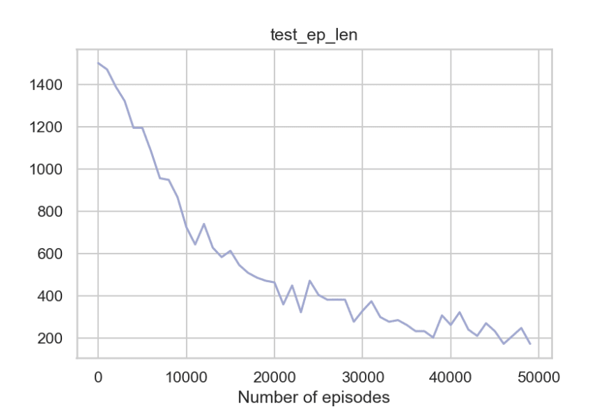
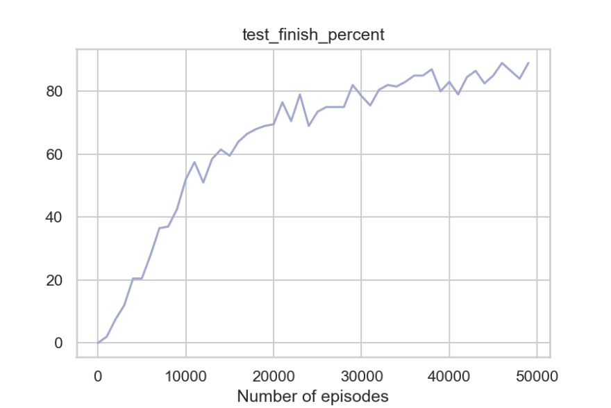
from collections import Counter, dequeimport random def bellman_update(q_table, state, action, next_state, reward): """ Function to perform q-value update as per bellman equation. """ # Get the old q_value old_q_value = q_table[state, action] # Find the maximum q_value for the actions in next state next_max = np.max(q_table[next_state]) # Calculate the new q_value as per the equation new_q_value = (1 - alpha) * old_q_value + alpha * (reward + gamma * next_max) # Finally, update the q_value q_table[state, action] = new_q_valuedef update(q_table, env, state): """ Selects an action according to epsilon greedy method, performs it, and the calls bellman update to update the Q-values. """ if random.uniform(0, 1) > epsilon: action = env.action_space.sample() else: action = np.argmax(q_table[state]) next_state, reward, done, info = env.step(action) bellman_update(q_table, state, action, next_state, reward) return next_state, reward, done, infodef train_agent( q_table, env, num_episodes, log_every=50000, running_metrics_len=50000, evaluate_every=1000, evaluate_trials=200): """ This is the training logic. It takes input as a q-table, the environment. The training is done for num_episodes episodes. The results are logged preiodcially. We also record some useful metrics like average reward in last 50k timesteps, the average length of last 50 episodes and so on. These are helpful to gauge how the algorithm is performing over time. After every few episodes of training. We run evaluation routine, where we just "exploit" i.e. rely on the q-table so far and see how well the agent has learned so far. Over the time, the results should get better until the q-table starts converging, after which, there's negligible change in the results. """ rewards = deque(maxlen=running_metrics_len) episode_lengths = deque(maxlen=50) total_timesteps = 0 metrics = {} for i in range(num_episodes): epochs = 0 state = env.reset() num_penalties, reward= 0, 0 done = False while not done: state, reward, done, info = update(q_table, env, state) rewards.append(reward) epochs += 1 total_timesteps += 1 if total_timesteps % log_every == 0: rd = Counter(rewards) avg_ep_len = np.mean(episode_lengths) zeroes, fill_percent = calculate_q_table_metrics(q_table) print(f'Current Episode: {i}') print(f'Reward distribution: {rd}') print(f'Last 10 episode lengths (avg: {avg_ep_len})') print(f'{zeroes} Q table zeroes, {fill_percent} percent filled') episode_lengths.append(epochs) if i % evaluate_every == 0: print('===' * 10) print(f"Running evaluation after {i} episodes") finish_percent, avg_time, penalties = evaluate_agent(q_table, env, evaluate_trials) print('===' * 10) rd = Counter(rewards) avg_ep_len = float(np.mean(episode_lengths)) zeroes, fill_percent = calculate_q_table_metrics(q_table) metrics[i] = { 'train_reward_distribution': rd, 'train_ep_len': avg_ep_len, 'fill_percent': fill_percent, 'test_finish_percent': finish_percent, 'test_ep_len': avg_time, 'test_penalties': penalties } print("Training finished.") return q_table, metricsdef calculate_q_table_metrics(grid): """ This function counts what perecentage of cells in the q-table are non-zero. Note: There are certain state-action combinations that are illegal, so the table might never be full. """ r, c = grid.shape total = r * c count = 0 for row in grid: for cell in row: if cell == 0: count += 1 fill_percent = (total - count) / total * 100.0 return count, fill_percentdef evaluate_agent(q_table, env, num_trials): """ The routine to evaluate an agent. It simply exploits the q-table and records the performance metrics. """ total_epochs, total_penalties, total_wins = 0, 0, 0 for _ in range(num_trials): state = env.reset() epochs, num_penalties, wins = 0, 0, 0 done = False while not done: next_action = np.argmax(q_table[state]) state, reward, done, _ = env.step(next_action) if reward < -2: num_penalties += 1 elif reward > 10: wins += 1 epochs += 1 total_epochs += epochs total_penalties += num_penalties total_wins += wins average_penalties, average_time, complete_percent = compute_evaluation_metrics(num_trials,total_epochs,total_penalties,total_wins) print_evaluation_metrics(average_penalties,average_time,num_trials,total_wins) return complete_percent, average_time, average_penaltiesdef print_evaluation_metrics(average_penalties, average_time, num_trials, total_wins): print("Evaluation results after {} trials".format(num_trials)) print("Average time steps taken: {}".format(average_time)) print("Average number of penalties incurred: {}".format(average_penalties)) print(f"Had {total_wins} wins in {num_trials} episodes")def compute_evaluation_metrics(num_trials, total_epochs, total_penalties, total_wins): average_time = total_epochs / float(num_trials) average_penalties = total_penalties / float(num_trials) complete_percent = total_wins / num_trials * 100.0 return average_penalties, average_time, complete_percentimport numpy as np# The hyper-parameters of Q-learningalpha = 0.1 # learning rategamma = 0.7 # discout factorepsilon = 0.2env = gym.make('DualTaxi-v1')num_episodes = 50000# Initialize a q-table full of zeroesq_table = np.zeros([env.observation_space.n, env.action_space.n])q_table, metrics = train_agent(q_table, env, num_episodes) # Get back trained q-table and metricsTotal encoded states are 6144==============================Running evaluation after 0 episodesEvaluation results after 200 trialsAverage time steps taken: 1500.0Average number of penalties incurred: 1500.0Had 0 wins in 200 episodes==============================----------------------------Skipping intermediate output----------------------------==============================Running evaluation after 49000 episodesEvaluation results after 200 trialsAverage time steps taken: 210.315Average number of penalties incurred: 208.585Had 173 wins in 200 episodes==============================Current Episode: 49404Reward distribution: Counter({-3: 15343, -12: 12055, -4: 11018, -11: 4143, -20: 3906, -30: 1266, -2: 1260, 99: 699, -10: 185, 90: 125})Last 10 episode lengths (avg: 63.0)48388 Q table zeroes, 78.12319155092592 percent filledTraining finished.I have skipped the intermediate output on purpose, you can check this pastebin if you're interested in full output.
Competitive Approach
The steps for this are similar to the cooperative approach, with the differnce that now we have multiple Q-tables to update.
- Initialize the Q-table 1 and 2 for both the agents by all zeros. The size of each Q-table is
state_space_size x sqrt(action_space_size). - Decide between exploration and exploitation based on the epsilon value.
- Exploration: For each state, select any one among all possible actions for the current state (S).
- Exploitation: For all possible actions from the state (S') select the one with the highest Q-value in the Q-tables of respective agents.
- Transition to the next state (S') as a result of that combined action (a1, a2).
- Update Q-table values for both the agents using the update equation and respective rewards & actions.
- If the episode is over (i.e. goal state is reached), reset the environment for next iteration.
- Keep repeating steps 2 to 7 until we start seeing decent results in the performance.
def update_multi_agent(q_table1, q_table2, env, state):    """    Same as update method discussed in the last section, just modified for two independent q-tables.    """    if random.uniform(0, 1) > epsilon:        action = env.action_space.sample()        action1, action2 = env.decode_action(action)    else:        action1 = np.argmax(q_table1[state])        action2 = np.argmax(q_table2[state])        action = env.encode_action(action1, action2)    next_state, reward, done, info = env.step(action)    reward1, reward2 = reward    bellman_update(q_table1, state, action1, next_state, reward1)    bellman_update(q_table2, state, action1, next_state, reward2)    return next_state, reward, done, infodef train_multi_agent(        q_table1, q_table2, env, num_episodes, log_every=50000, running_metrics_len=50000,        evaluate_every=1000, evaluate_trials=200):    """    Same as train method discussed in the last section, just modified for two independent q-tables.    """    rewards = deque(maxlen=running_metrics_len)    episode_lengths = deque(maxlen=50)    total_timesteps = 0    metrics = {}    for i in range(num_episodes):        epochs = 0        state = env.reset()        done = False        while not done:            # Modification here            state, reward, done, info = update_multi_agent(q_table1, q_table2, env, state)            rewards.append(sum(reward))            epochs += 1            total_timesteps += 1            if total_timesteps % log_every == 0:                rd = Counter(rewards)                avg_ep_len = np.mean(episode_lengths)                zeroes1, fill_percent1 = calculate_q_table_metrics(q_table1)                zeroes2, fill_percent2 = calculate_q_table_metrics(q_table2)                print(f'Current Episode: {i}')                print(f'Reward distribution: {rd}')                print(f'Last 10 episode lengths (avg: {avg_ep_len})')                print(f'{zeroes1} Q table 1 zeroes, {fill_percent1} percent filled')                print(f'{zeroes2} Q table 2 zeroes, {fill_percent2} percent filled')        episode_lengths.append(epochs)        if i % evaluate_every == 0:            print('===' * 10)            print(f"Running evaluation after {i} episodes")            finish_percent, avg_time, penalties = evaluate_multi_agent(q_table1, q_table2, env, evaluate_trials)            print('===' * 10)            rd = Counter(rewards)            avg_ep_len = float(np.mean(episode_lengths))            zeroes1, fill_percent1 = calculate_q_table_metrics(q_table1)            zeroes2, fill_percent2 = calculate_q_table_metrics(q_table2)            metrics[i] = {                    'train_reward_distribution': rd,                    'train_ep_len': avg_ep_len,                    'fill_percent1': fill_percent1,                    'fill_percent2': fill_percent2,                    'test_finish_percent': finish_percent,                    'test_ep_len': avg_time,                    'test_penalties': penalties            }    print("Training finished.
")    return q_table1, q_table2, metricsdef evaluate_multi_agent(q_table1, q_table2, env, num_trials):    """    Same as evaluate method discussed in last section, just modified for two independent q-tables.    """    total_epochs, total_penalties, total_wins = 0, 0, 0    for _ in range(num_trials):        state = env.reset()        epochs, num_penalties, wins = 0, 0, 0        done = False        while not done:            # Modification here            next_action = env.encode_action(                np.argmax(q_table1[state]),                np.argmax(q_table2[state]))            state, reward, done, _ = env.step(next_action)            reward = sum(reward)            if reward < -2:                num_penalties += 1            elif reward > 10:                wins += 1            epochs += 1        total_epochs += epochs        total_penalties += num_penalties        total_wins += wins    average_penalties, average_time, complete_percent = compute_evaluation_metrics(num_trials,total_epochs,total_penalties,total_wins)    print_evaluation_metrics(average_penalties,average_time,num_trials,total_wins)    return complete_percent, average_time, average_penalties
# The hyperparameter of Q-learningalpha = 0.1gamma = 0.8epsilon = 0.2env_c = gym.make('DualTaxi-v1', competitive=True)num_episodes = 50000q_table1 = np.zeros([env_c.observation_space.n, int(np.sqrt(env_c.action_space.n))])q_table2 = np.zeros([env_c.observation_space.n, int(np.sqrt(env_c.action_space.n))])q_table1, q_table2, metrics_c = train_multi_agent(q_table1, q_table2, env_c, num_episodes)Total encoded states are 6144==============================Running evaluation after 0 episodesEvaluation results after 200 trialsAverage time steps taken: 1500.0Average number of penalties incurred: 1500.0Had 0 wins in 200 episodes==============================----------------------------Skipping intermediate output----------------------------==============================Running evaluation after 48000 episodesEvaluation results after 200 trialsAverage time steps taken: 323.39Average number of penalties incurred: 322.44Had 158 wins in 200 episodes==============================Current Episode: 48445Reward distribution: Counter({-12: 13993, -3: 12754, -4: 11561, -20: 3995, -11: 3972, -30: 1907, -10: 649, -2: 524, 90: 476, 99: 169})Last 10 episode lengths (avg: 78.08)8064 Q table 1 zeroes, 78.125 percent filled8064 Q table 2 zeroes, 78.125 percent filled==============================Running evaluation after 49000 episodesEvaluation results after 200 trialsAverage time steps taken: 434.975Average number of penalties incurred: 434.115Had 143 wins in 200 episodes==============================Current Episode: 49063Reward distribution: Counter({-3: 13928, -12: 13605, -4: 10286, -11: 4542, -20: 3917, -30: 1874, -10: 665, -2: 575, 90: 433, 99: 175})Last 10 episode lengths (avg: 75.1)8064 Q table 1 zeroes, 78.125 percent filled8064 Q table 2 zeroes, 78.125 percent filledCurrent Episode: 49706Reward distribution: Counter({-12: 13870, -3: 13169, -4: 11054, -11: 4251, -20: 3985, -30: 1810, -10: 704, -2: 529, 90: 436, 99: 192})Last 10 episode lengths (avg: 76.12)8064 Q table 1 zeroes, 78.125 percent filled8064 Q table 2 zeroes, 78.125 percent filledTraining finished.I have skipped the intermediate output on purpose, you can check this pastebin if you're interested in full output.
Evaluating the performance
If you observed the code carefully, the train functions returned q-tables as well as some metrics. We can use the q-table now for taking agent's actions, and see how intelligent it has become. Also, we'll try to plot these metrics to visualize how the training progressed.
from collections import defaultdictimport matplotlib.pyplot as plt # import seaborn as pltdef plot_metrics(m): """ Plotting various metrics over the number of episodes. """ ep_nums = list(m.keys()) series = defaultdict(list) for ep_num, metrics in m.items(): for metric_name, metric_val in metrics.items(): t = type(metric_val) if t in [float, int, np.float64]: series[metric_name].append(metric_val) for m_name, values in series.items(): plt.plot(ep_nums, values) plt.title(m_name) plt.xlabel('Number of episodes') plt.show()def play(q_table, env, num_episodes): for i in range(num_episodes): state = env.reset() done = False while not done: next_action = np.argmax(q_table[state]) state, reward, done, _ = env.step(next_action)def play_multi(q_table1, q_table2, env, num_episodes): """ Capture frames by playing using the two q-tables. """ for i in range(num_episodes): state = env.reset() done = False while not done: next_action = env.encode_action( np.argmax(q_table1[state]), np.argmax(q_table2[state])) state, reward, done, _ = env.step(next_action)plot_metrics(metrics)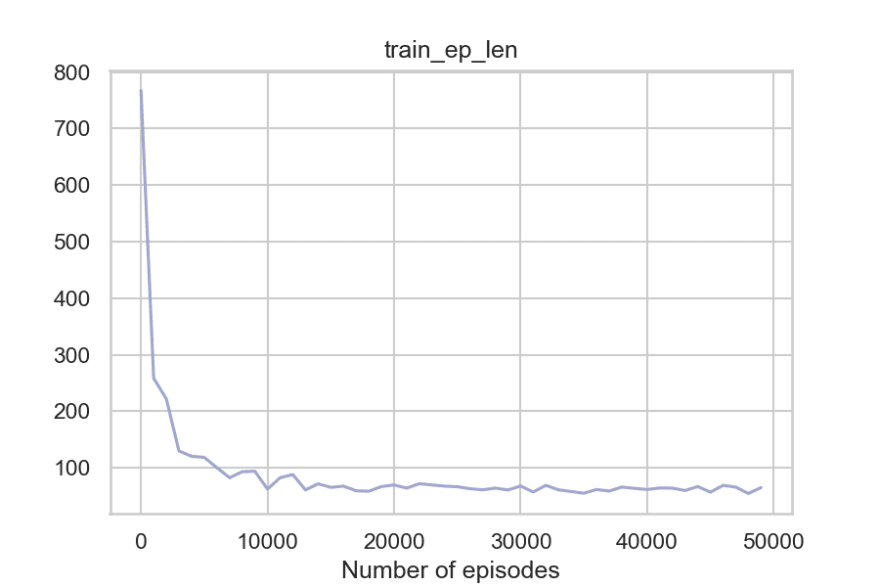


frames = play(q_table, env, 10)print_frames(frames)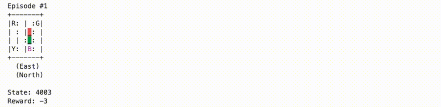
plot_metrics(metrics_c)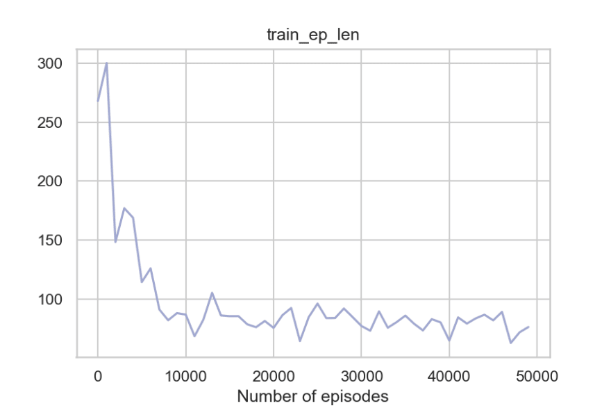


print_frames(play_multi(q_table1, q_table2, env_c, 10))
Some observations
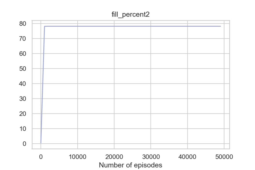
- While Q-learning agent commits errors initially during exploration but once it has explored enough (seen most of the states), it starts to act wisely.
- Both the approaches did fairly well. However, in relative comparison, the cooperative approach seem to perform better. The plots of competitive approach are more volatile.
- It took around 2000 episodes for agents to explore most of the possible state-action pairs. Note that not state-action pairs are feasible because some states aren't legal (for example, states where both the taxis are at same location aren't possible).
- As the training progressed the number of penalties reduced. They didn't reduce completely because of the epsilon (we're still exploring based on the epsilon value during training).
- The episode length kept decreasing, which means the taxis were able to pickup and drop the passenger faster because of the new learned knowledge in q-tables.
So to summarize, the agent is able to get around the walls, pick the passengers, take less penalties, and reach the destination timely. And the fact that the code where q-learning update happens is merely around 20-30 lines of Python code makes it even more impressive.
From what we've discussed so far in the post, it's likely that you have a fair bit of intution about how Reinforcement Learning works. Now in the last few sections we will dip our toes in some broader level ideas and concepts that might be relevant to you when exploring Reinforcement Learning further. Let's start with the common challenges of Reinforcement Learning first,
Common challenges while applying Reinforcement learning
Finiding the right Hyperparameters
You might be wondering how did I decide values of alpha, gamma, and epsilon. In the above program, it was mostly based on intuition from my past experience and some "hit and trial". This goes a long way, but there are also some techniques to come up with good values. The process in itself is sometimes referred to as Hyperparamter tuning or Hyperparameter optimization.
Tuning the hyperparameters
A simple way to programmatically come up with the best set of values of the hyperparameter is to create a comprehensive search function that selects the parameters that would result in best agent performance. A more sophisticated way to get the right combination of hyperparameter values would be to use Genetic Algorithms. Also, it is a common practice to make these parameters dynamic instead of fixed values. For example, in our case, all of the three hyperparmeters can be configured to decrease over time because as the agent continues to learn, it builds up more resilient priors.
Choosing the right algorithms
Q-learning is just one of the many Reinformcement Learning algorithms out there. There are multiple ways to classify Reinforcement Learning algorithms. The selection depends on various factors including the nature of the environment. For example, if the state space of action space is continuous instead of discrete (imagine that the environment now expects continuous degree values instead of discrete north / east / etc directions as actions, and the state space consists of more precise lat/lng location of taxis instead of grid coordinates), tabular Q-learning can't work. There are hacks to get around continuous spaces (like bucketing their range and making it discrete as a result), but these hacks fail too if the state space and action space gets too large. In those cases, it is preferred to use more generic algorithms, usually the ones that involve approximators like Neural Networks.
More often than not, in practice, the agent is trained with multiple algorithms initially to decide which algorithm would fit the best.
Reward Structure
It is important to think strategically about the rewards to be given to the agent. If the rewards are too sparse, the agent might have difficulty in learning. Poorly structured rewards can also lead to cases of non-convergence and situations in which agent gets stuck in local minima. For example, let's say the environment gave +1 reward for successfully picking up passenger, and no penalty for dropping the passenger. So it might happen, that the agent might end up repeatedly picking up and dropping a passenger to maximise it rewards. Similary, if we there was very high negative reward for picking up passenger, agent would eventually learn to not pick a passenger at all, and hence would never finish successfully.
The challenges of real world environments
Training an agent on an openAI gym environment is realtively easy because you get a lot of things out of the box. The real world, however, is a bit more unorganised. We sensors to ingest environment information and mechanism to translate it into something that can be fed to a Machine Learning algorithm. So such systems involve a lots of techniques overall aside from the learning algorithm. As a simple example, consider a general Reinforcement Learning agent that is being trained to play ATARI games. The information this agent needs to be passed is pixels on the screen. So we might have to use deep learning techniques (like Convolutional Neural Networks) to interpret the pixels on the screen and extract information out of the game (like scores) to enable the agent to interpret the game.
There's also a challenge of sample efficiency. Since the state spaces and action spaces might be continuous and have big ranges, it becomes critical to achieve a decent sample efficiency that makes Reinforcement Learning feasible. If the algorithm needs high number of episodes (high enough that we cannot make it to produce results in reasonable amount of time), then Reinforcement Learning becomes impractical.
Respecting the theoretical boundaries
It is easy to sometimes get carried away and see Reinforcement Learning to be the solution of most problems. It helps to have a theoretical understanding of how these algorithm works and fundamental concepts like Markov Decision Processes and awareness of the state of the art algorithms to have a better intution about what can and what can't be solved using present-day Reinforcement Learning algorithms.
Wrapping up
In this tutorial, we began with understanding Reinforcement Learning with the help of real-world analogies. Then we learned about some fundamental conepts like state, action, and rewards. Next, we went over the process of framing a problem such that we can traing an agent through Reinforcement Learning algorithms to solve it.
We took Self-driving taxi as our reference problem for the rest of the tutorial. We then used OpenAL's gym module in python to provide us with a related environment, where we can develop our agent and evaluate it. Then we observed how terrible our agent was without using any algorithm to play the game, so we went ahead to implement the Q-learning algorithm from scratch.
We then introduced Q-learning, and went over the steps to use it for our environment. We came up with two approaches (cooperative and competitive). We then evaluated the Q-learning results, and saw how the agent's performance improved significantly after Q-learning.
As mentioned in beginning, Reinforcement learning is not just limited to openAI gym environments and games. It is also used for managing portfolio and finances, for making humanoid robots, for manufacturing and inventory management, to develop general AI agents (agents that can perform multiple things with a single algorithm, like same agent playing multiple Atari games).
Appendix
Further reading
- "Reinforcement Learning: An Introduction" Book by Andrew Barto and Richard S. Sutton. Most popular book about Reinforcement Learning out there. Highly recommended if you're planning to dive deep into the field.
- Lectures by David Silver (also available on YouTube). Another great resource if you're more into learning from videos than books.
- Tutorial series on medium on Reinforcement learning using Tensorflow by Arthur Juliani.
- Some interesting topics related to Multi Agent environments,
- Friend and foe Q-learning in general-sum games
- Game theory concepts like
- Strictly dominant strategies
- Nash equilibrium
- Shapely values for reward distribution
Visualising the transition table of our dual taxi enviroment
The following is an attempt to visualize the internal tranistion table of our environment in a human readable way. The source of this information is the env.P object which contains a mapping of the form
current_state : action_taken: [(transition_prob, next_state, reward, done)], this is all the info we need to simulate the environment and this is what we can use to create the transition table.
env.P # First let's take a peek at this object{0: { 0: [(1.0, 0, -30, False)], 1: [(1.0, 1536, -0.5, True)], 2: [(1.0, 1560, -0.5, True)], 3: [(1.0, 1536, -0.5, True)], 4: [(1.0, 1536, -0.5, True)], 5: [(1.0, 1536, -0.5, True)], 6: [(1.0, 96, -0.5, True)], 7: [(1.0, 0, -30, False)], 8: [(1.0, 24, -0.5, True)], 9: [(1.0, 0, -30, False)], 10: [(1.0, 0, -30, False)], 11: [(1.0, 0, -30, False)], 12: [(1.0, 480, -0.5, True)], 13: [(1.0, 384, -0.5, True)], 14: [(1.0, 0, -30, False)], 15: [(1.0, 384, -0.5, True)], 16: [(1.0, 384, -0.5, True)], 17: [(1.0, 384, -0.5, True)], 18: [(1.0, 96, -0.5, True)], 19: [(1.0, 0, -30, False)], 20: [(1.0, 24, -0.5, True)], 21: [(1.0, 0, -30, False)], 22: [(1.0, 0, -30, False)], 23: [(1.0, 0, -30, False)], 24: [(1.0, 96, -0.5, True)], 25: [(1.0, 0, -30, False)], 26: [(1.0, 24, -0.5, True)], 27: [(1.0, 0, -30, False)], 28: [(1.0, 0, -30, False)], 29: [(1.0, 0, -30, False)], 30: [(1.0, 96, -0.5, True)], 31: [(1.0, 0, -30, False)], 32: [(1.0, 24, -0.5, True)], 33: [(1.0, 0, -30, False)], 34: [(1.0, 0, -30, False)], 35: [(1.0, 0, -30, False)]}, 1: {0: [(1.0, 1, -30, False)], 1: [(1.0, 1537, -0.5, True)], 2: [(1.0, 1561, -0.5, True)], 3: [(1.0, 1537, -0.5, True)], 4: [(1.0, 1537, -0.5, True)], 5: [(1.0, 1537, -0.5, True)], 6: [(1.0, 97, -0.5, True)], 7: [(1.0, 1, -30, False)], 8: [(1.0, 25, -0.5, True)], 9: [(1.0, 1, -30, False)], 10: [(1.0, 1, -30, False)], 11: [(1.0, 1, -30, False)], 12: [(1.0, 481, -0.5, True)], 13: [(1.0, 385, -0.5, True)], 14: [(1.0, 1, -30, False)], 15: [(1.0, 385, -0.5, True)], 16: [(1.0, 385, -0.5, True)], 17: [(1.0, 385, -0.5, True)], 18: [(1.0, 97, -0.5, True)], 19: [(1.0, 1, -30, False)], 20: [(1.0, 25, -0.5, True)], 21: [(1.0, 1, -30, False)], 22: [(1.0, 1, -30, False)], 23: [(1.0, 1, -30, False)], 24: [(1.0, 97, -0.5, True)], 25: [(1.0, 1, -30, False)], 26: [(1.0, 25, -0.5, True)], 27: [(1.0, 1, -30, False)], 28: [(1.0, 1, -30, False)], 29: [(1.0, 1, -30, False)], 30: [(1.0, 97, -0.5, True)], 31: [(1.0, 1, -30, False)], 32: [(1.0, 25, -0.5, True)], 33: [(1.0, 1, -30, False)], 34: [(1.0, 1, -30, False)], 35: [(1.0, 1, -30, False)]},# omitting the whole output because it's very long! Now, let's put some code together to convert this information in more readable tabular form.
! pip install pandasimport pandas as pdtable = []env_c = gym.make('DualTaxi-v1', competitive=True)def state_to_human_readable(s): passenger_loc = ['R', 'G', 'B', 'Y', 'T1', 'T2'][s[2]] destination = ['R', 'G', 'B', 'Y'][s[3]] return f'Taxi 1: {s[0]}, Taxi 2: {s[1]}, Pass: {passenger_loc}, Dest: {destination}'def action_to_human_readable(a): actions = 'NSEWPD' return actions[a[0]], actions[a[1]]for state_num, transition_info in env_c.P.items(): for action, possible_transitions in transition_info.items(): transition_prob, next_state, reward, done = possible_transitions[0] table.append({ 'State': state_to_human_readable(list(env.decode(state_num))), 'Action': action_to_human_readable(env.decode_action(action)), 'Probablity': transition_prob, 'Next State': state_to_human_readable(list(env.decode(next_state))), 'Reward': reward, 'Is over': done, })pd.DataFrame(table)| State | Action | Probablity | Next State | Reward | Is over | |
|---|---|---|---|---|---|---|
| 0 | Taxi 1: (0, 0), Taxi 2: (0, 0), Pass: R, Dest: R | (N, N) | 1.0 | Taxi 1: (0, 0), Taxi 2: (0, 0), Pass: R, Dest: R | (-15, -15) | False |
| 1 | Taxi 1: (0, 0), Taxi 2: (0, 0), Pass: R, Dest: R | (N, S) | 1.0 | Taxi 1: (1, 0), Taxi 2: (0, 0), Pass: R, Dest: R | (-0.5, 0) | True |
| 2 | Taxi 1: (0, 0), Taxi 2: (0, 0), Pass: R, Dest: R | (N, E) | 1.0 | Taxi 1: (1, 0), Taxi 2: (0, 1), Pass: R, Dest: R | (-0.5, 0) | True |
| 3 | Taxi 1: (0, 0), Taxi 2: (0, 0), Pass: R, Dest: R | (N, W) | 1.0 | Taxi 1: (1, 0), Taxi 2: (0, 0), Pass: R, Dest: R | (-0.5, 0) | True |
| 4 | Taxi 1: (0, 0), Taxi 2: (0, 0), Pass: R, Dest: R | (N, P) | 1.0 | Taxi 1: (1, 0), Taxi 2: (0, 0), Pass: R, Dest: R | (-0.5, 0) | True |
| ... | ... | ... | ... | ... | ... | ... |
| 221179 | Taxi 1: (3, 3), Taxi 2: (3, 3), Pass: T2, Dest: Y | (D, S) | 1.0 | Taxi 1: (3, 3), Taxi 2: (2, 3), Pass: T2, Dest: Y | (-0.5, 0) | True |
| 221180 | Taxi 1: (3, 3), Taxi 2: (3, 3), Pass: T2, Dest: Y | (D, E) | 1.0 | Taxi 1: (3, 3), Taxi 2: (3, 3), Pass: T2, Dest: Y | (-15, -15) | False |
| 221181 | Taxi 1: (3, 3), Taxi 2: (3, 3), Pass: T2, Dest: Y | (D, W) | 1.0 | Taxi 1: (3, 3), Taxi 2: (3, 2), Pass: T2, Dest: Y | (-0.5, 0) | True |
| 221182 | Taxi 1: (3, 3), Taxi 2: (3, 3), Pass: T2, Dest: Y | (D, P) | 1.0 | Taxi 1: (3, 3), Taxi 2: (3, 3), Pass: T2, Dest: Y | (-15, -15) | False |
| 221183 | Taxi 1: (3, 3), Taxi 2: (3, 3), Pass: T2, Dest: Y | (D, D) | 1.0 | Taxi 1: (3, 3), Taxi 2: (3, 3), Pass: T2, Dest: Y | (-15, -15) | False |
221184 rows 6 columns
Bloopers
In retrospect, the hardest part of writing this post was to get the dual-taxi-environment working. There were so many moments like below,

It took a lot of trial and errors (tweaking rewards, updating rules for situations like collision, reducing state space) to get to a stage where the solutions for competitive set up were converging. The feeling when the solution converges for the first time is very cool. So if you have some free time, I'd recommend you to hack up an environment yourself (the first time I tried q-learning was with a snake-apple game I developed using pygame), and try to solve it with Reinforcement Learning. Trust me, you'll be humbled and learn lots of interesting things along the way!
Original Link: https://dev.to/satwikkansal/a-gentle-introduction-to-reinforcement-learning-75h
Dev To
More About this Source Visit Dev To