Linear Regression is the genesis of Machine Learning for many beginners. People start learning ML from Linear Regression and then proceed to make awesome projects. If someone claims to be ignorant of Machine Learning's awesomeness he/she is surely living under the rock.

Let's start with the basic concept of Machine Learning and take a tour in the world of statistics and Machine learning. Linear Regression basically means fitting a line for a set of points which represent the features.

The hypothesis function represents the equation of the line to be fitted. Here theta-0 and theta-1 represent the parameters of the regression line. In the equation of line y = mx + c, m is slope and c is the y-intercept of the line. In the given equation theta-0 is the y-intercept and theta-1 is the slope of the regression line.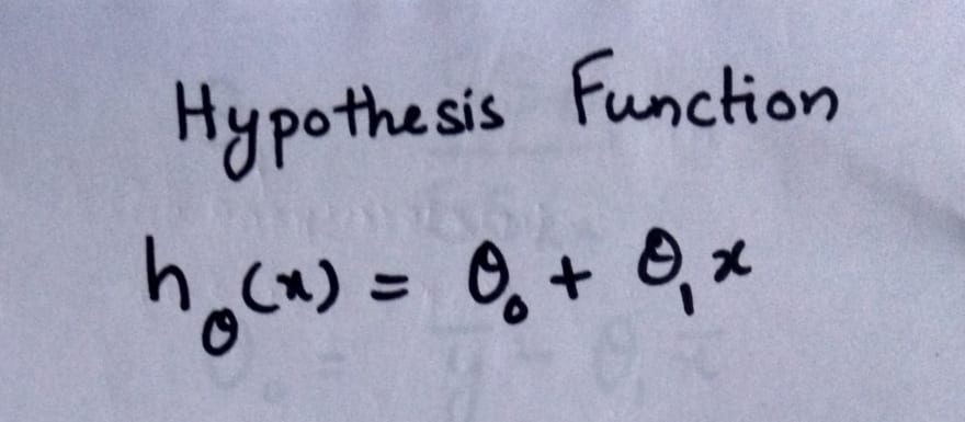

NOTE- Here we are dealing with a single independent variable x.

Cost function is the function we have to minimize to get the appropriate and optimum line. Here the difference between h-theta and y is known as error. We take the mean of squared error as the cost function.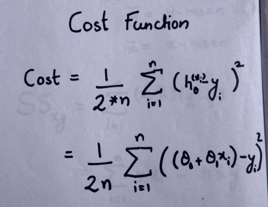

To calculate the value of theta-0 and theta-1 the equations are given below. We calculate the values using these equations and this method is known as Least Square estimation method.

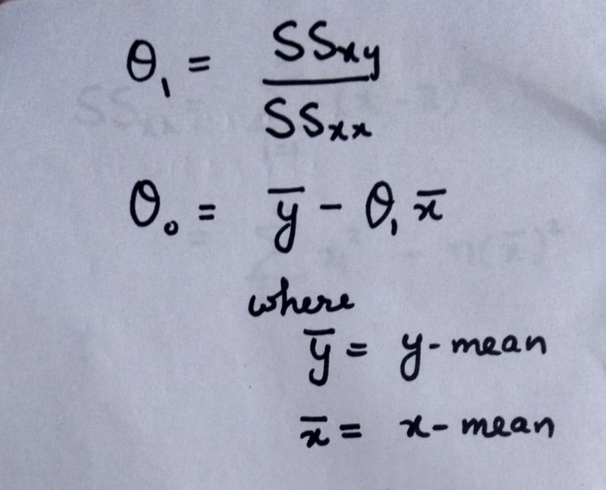
Here we are representing the features(independent variables) for each sample as x-i and their mean as x-bar. Also, the output(dependent variables) for each sample are represented as y-i and their mean as y-bar. The total number of samples is n.

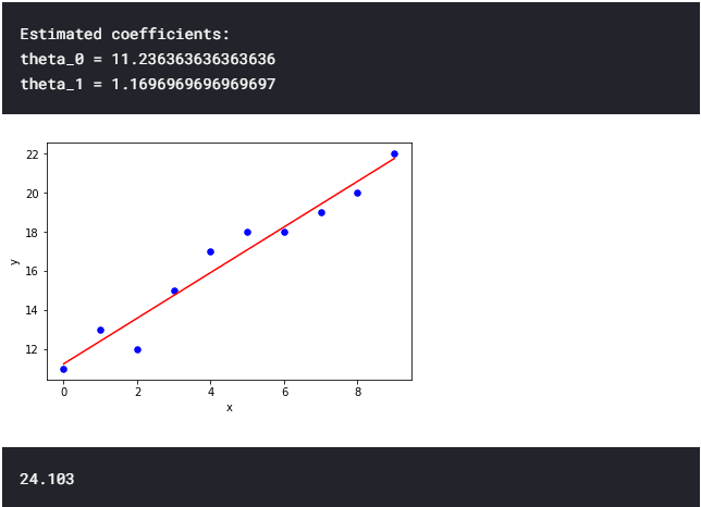
After applying the above equations we can find the best fitting line for the points scattered. The python code for this is represented below.

import numpy as np import matplotlib.pyplot as plt def estimate_coef(x, y):     n = np.size(x)     m_x, m_y = np.mean(x), np.mean(y)     SS_xy = np.sum(y*x) - n*m_y*m_x     SS_xx = np.sum(x*x) - n*m_x*m_x     theta_1 = SS_xy / SS_xx     theta_0 = m_y - theta_1*m_x     return(theta_0, theta_1) def plot_regression_line(x, y, theta):     plt.scatter(x, y, color = "b",marker = "o", s = 30)     y_pred = theta[0] + theta[1]*x     plt.plot(x, y_pred, color = "r")     plt.xlabel('x')     plt.ylabel('y')     plt.show() x = np.array([0, 1, 2, 3, 4, 5, 6, 7, 8, 9]) y = np.array([11 ,13, 12, 15, 17, 18, 18, 19, 20, 22]) theta = estimate_coef(x, y) print("Estimated coefficients:\ntheta_0 = {} \ntheta_1 = {}".format(theta[0], theta[1])) plot_regression_line(x, y, theta) print(round(theta[0]+ theta[1]*11,4))

Output

The methods are:-

• Using scikit-learn library's built-in LinearRegression function
• Using Gradient Descent Method
• Using Moore-Penrose inverse method.

Linear Regression using scikit learn

The simplest method is using built-in library function. The code for which is given below. The dataset used is same as the above used dataset. After fitting the line we are finding the value of y for x = 11. We will be using the same dataset and input value for all the different methods which will be used.

LinearRegression() function takes the input parameters in the form of sparse matrices of shape (n_samples, n_features) and (n_samples, n_targets).

import numpy as np;from sklearn.linear_model import LinearRegression;x = np.array([[0], [1],[2], [3], [4], [5], [6], [7], [8], [9]]) y = np.array([[11], [13], [12], [15], [17], [18], [18], [19], [20], [22]]) LR=LinearRegression()LR.fit(x,y)b=LR.predict(np.array([[11]]))print(round(b[0][0],4))

Output

24.103

Linear Regression using Gradient Descent

Gradient Descent is one of the most used methods to optimize different convex functions in Machine Learning. Since we know that the cost function which is the same as the cost function given in the Least Square Method is convex we will be using Gradient Descent to solve the problem. We have to minimize the cost function to find the value of Theta in the regression line.

The method of gradient descent can be represented as follow

Since we cannot update the values of theta-0 and theta-1 simultaneously we use temporary variables

import numpy as np;from matplotlib import pyplot as plt;# Function for cost functiondef cost(z,theta,y):    m,n=z.shape;    htheta = z.dot(theta.transpose())    cost = ((htheta - y)**2).sum()/(2.0 * m);    return cost;def gradient_descent(z,theta,alpha,y,itr):    cost_arr=[]    m,n=z.shape;    count=0;    htheta = z.dot(theta.transpose())    while count<itr:        htheta = z.dot(theta.transpose())        a=(alpha/m)        # Using temporary variables for simultaneous updation of variables        temp0=theta[0,0]-a*(htheta-y).sum();        temp1=theta[0,1]-a*((htheta-y)*(z[::,1:])).sum();        theta[0,0]=temp0;        theta[0,1]=temp1;        cost_arr.append(float(cost(z,theta,y)));        count+=1;    cost_log = np.array(cost_arr);    plt.plot(np.linspace(0, itr, itr, endpoint=True), cost_log)    plt.xlabel("No. of iterations")    plt.ylabel("Error Function value")    plt.show()    return theta;x = np.array([[0], [1],[2], [3], [4], [5], [6], [7], [8], [9]]) y = np.array([[11], [13], [12], [15], [17], [18], [18], [19], [20], [22]]) m,n=x.shape;z=np.ones((m,n+1),dtype=int);z[::,1:]=x;theta=np.array([[21,2]],dtype=float)theta_minimised=gradient_descent(z,theta,0.01,y,10000)new_x=np.array([1,11])predicted_y=new_x.dot(theta_minimised.transpose())print(round(predicted_y[0],4));

Output

Linear Regression using Pseudo Inverse Method

The equation for finding theta in case of Moore-penrose inverse method(Pseudo inverse method) is given below.

And it is implemented in the code given below.

import numpy as np;# Input Matrixx= np.array([[0], [1],[2], [3], [4], [5], [6], [7], [8], [9]]) # Output Matrixy= np.array([[11], [13], [12], [15], [17], [18], [18], [19], [20], [22]]) m,n=x.shape;# Adding extra ones for the theta-0 or bias termz=np.ones((m,n+1),dtype=int);z[:,1:]=x; # z is Input matrix with added 1smat=np.matmul(z.transpose(),z); # product of z and z transposematinv=np.linalg.inv(mat) #inverse of above productval=np.matmul(matinv,z.transpose()) # Product of inverse and z transposetheta=np.matmul(val,y) # Value of theta by multiplying value calculated above to ynew_x=np.array([1,11]);predicted_y=new_x.dot(theta);print(round(predicted_y[0],4));

Output

24.103

After learning linear regression let's apply it on some real Dataset. The dataset we will use is Boston dataset.

It has 506 samples and 13 features and one column as output column. The 14 column is output. Here is a sample code for Boston Dataset.

Have a little bit of patience for the Repl editor. Hope you liked the article.