Handling Imbalanced Datasets with SMOTE in Python

Close your eyes.

Now imagine a perfect data world. What do you see? What do you wish to see? Exactly, me too. A flawlessly balanced dataset. A collection of data whose labels form a magnificent 1:1 ratio: 50% of this, 50% of that; not a bit to the left, nor a bit to the right. Just perfectly balanced, as all things should be. Now open your eyes, and come back to the real world.

The opposite of a pure balanced dataset is a highly imbalanced dataset, and unfortunately for us, these are quite common. An imbalanced dataset is a dataset where the number of data points per class differs drastically, resulting in a heavily biased machine learning model that wont be able to learn the minority class. When this imbalanced ratio is not so heavily skewed toward one class, such dataset is not that horrible, since many machine learning models can handle them.

Nevertheless, there are some extreme cases in which the class ratio is just wrong, for example, a dataset where 95% of the labels belong to class A, while the remaining 5% fall under class B a ratio not so rare in use cases such as fraud detection. In these extreme cases, the ideal course of action would be to collect more data.

However, this is typically not feasible; in fact, its costly, time-consuming and in most cases, impossible. Luckily for us, theres an alternative known as oversampling. Oversampling involves using the data we currently have to create more of it.

What is data oversampling?

Data oversampling is a technique applied to generate data in such a way that it resembles the underlying distribution of the real data. In this article, I explain how we can use an oversampling technique called Synthetic Minority Over-Sampling Technique or SMOTE to balance out our dataset.

What is SMOTE?

SMOTE is an oversampling algorithm that relies on the concept of nearest neighbors to create its synthetic data. Proposed back in 2002 by Chawla et. al., SMOTE has become one of the most popular algorithms for oversampling.

The simplest case of oversampling is simply called oversampling or upsampling, meaning a method used to duplicate randomly selected data observations from the outnumbered class.

Oversamplings purpose is for us to feel confident the data we generate are real examples of already existing data. This inherently comes with the issue of creating more of the same data we currently have, without adding any diversity to our dataset, and producing effects such as overfitting.

Hence, if overfitting affects our training due to randomly generated, upsampled data or if plain oversampling is not suitable for the task at hand we could resort to another, smarter oversampling technique known as synthetic data generation.

Synthetic data is intelligently generated artificial data that resembles the shape or values of the data it is intended to enhance. Instead of merely making new examples by copying the data we already have (as explained in the last paragraph), a synthetic data generator creates data that is similar to the existing one. Creating synthetic data is where SMOTE shines.

How does SMOTE work?

To show how SMOTE works, suppose we have an imbalanced two-dimensional dataset, such as the one in the next image, and we want to use SMOTE to create new data points.

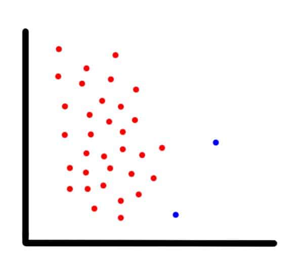
Example of an imbalanced dataset

For each observation that belongs to the under-represented class, the algorithm gets its K-nearest-neighbors and synthesizes a new instance of the minority label at a random location in the line between the current observation and its nearest neighbor.

In our example (shown in the next image), the blue encircled dot is the current observation, the blue non-encircled dot is its nearest neighbor, and the green dot is the synthetic one.

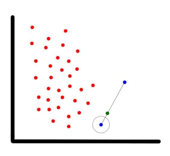
SMOTEs new synthetic data point

Now lets do it in Python.

SMOTE tutorial using imbalanced-learn

In this tutorial, I explain how to balance an imbalanced dataset using the package imbalanced-learn.

First, I create a perfectly balanced dataset and train a machine learning model with it which Ill call our base model. Then, Ill unbalance the dataset and train a second system which Ill call an imbalanced model.

Finally, Ill use SMOTE to balance out the dataset, followed by fitting a third model with it which Ill name the SMOTEd model. By training a new model at each step, Well be able to better understand how an imbalanced dataset can affect a machine learning system.

Base model

Example code for this article may be found at the Kite Blog repository.

For the initial task, Ill fit a support-vector machine (SVM) model using a created, perfectly balanced dataset. I chose this kind of model because of how easy it is to visualize and understand its decision boundary, namely, the hyperplane that separates one class from the other.

To generate a balanced dataset, Ill use scikit-learns make_classification function which creates n clusters of normally distributed points suitable for a classification problem.

My fake dataset consists of 700 sample points, two features, and two classes. To make sure each class is one blob of data, Ill set the parameter n_clusters_per_class to 1.

To simplify it, Ill remove the redundant features and set the number of informative features to 2. Lastly, Ill useflip_y=0.06 to reduce the amount of noise.

The following piece of code shows how we can create our fake dataset and plot it using Pythons Matplotlib.

import matplotlib.pyplot as pltimport pandas as pdfrom sklearn.datasets import make_classificationfrom imblearn.datasets import make_imbalance# for reproducibility purposesseed = 100# create balanced datasetX1, Y1 = make_classification(n_samples=700, n_features=2, n_redundant=0,                            n_informative=2, n_clusters_per_class=1,                            class_sep=1.0, flip_y=0.06, random_state=seed)plt.title('Balanced dataset')plt.xlabel('x')plt.ylabel('y')plt.scatter(X1[:, 0], X1[:, 1], marker='o', c=Y1,           s=25, edgecolor='k', cmap=plt.cm.coolwarm)plt.show()# concatenate the features and labels into one dataframedf = pd.concat([pd.DataFrame(X1), pd.DataFrame(Y1)], axis=1)df.columns = ['feature_1', 'feature_2', 'label']# save the dataset because we'll use it laterdf.to_csv('df_base.csv', index=False, encoding='utf-8')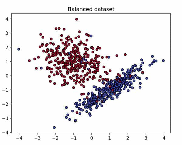

A balanced dataset

As you can see in the previous image, our balanced dataset looks tidy and well defined. So, if we fit an SVM model with this data (code below), how will the decision boundary look?

Since well be training several models and visualizing their hyperplanes, I wrote two functions that will be reused several times throughout the tutorial. The first one, train_SVM, is for fitting the SVM model, and it takes the dataset as a parameter.

The second function, plot_svm_boundary, plots the decision boundary of the SVM model. Its parameters also include the dataset and the caption of the plot.

These are the functions:

import matplotlib.pyplot as pltimport numpy as npimport pandas as pdfrom sklearn.svm import SVCdef train_SVM(df):   # select the feature columns   X = df.loc[:, df.columns != 'label']   # select the label column   y = df.label   # train an SVM with linear kernel   clf = SVC(kernel='linear')   clf.fit(X, y)   return clfdef plot_svm_boundary(clf, df, title):   fig, ax = plt.subplots()   X0, X1 = df.iloc[:, 0], df.iloc[:, 1]   x_min, x_max = X0.min() - 1, X0.max() + 1   y_min, y_max = X1.min() - 1, X1.max() + 1   xx, yy = np.meshgrid(np.arange(x_min, x_max, 0.02), np.arange(y_min, y_max, 0.02))   Z = clf.predict(np.c_[xx.ravel(), yy.ravel()])   Z = Z.reshape(xx.shape)   out = ax.contourf(xx, yy, Z, cmap=plt.cm.coolwarm, alpha=0.8)   ax.scatter(X0, X1, c=df.label, cmap=plt.cm.coolwarm, s=20, edgecolors='k')   ax.set_ylabel('y')   ax.set_xlabel('x')   ax.set_title(title)   plt.show()

To fit and plot the model, do the following:

df = pd.read_csv('df_base.csv', encoding='utf-8', engine='python')clf = train_SVM(df)plot_svm_boundary(clf, df, 'Decision Boundary of SVM trained with a balanced dataset')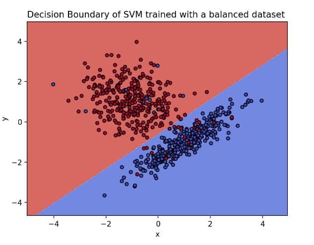

Blue dots on the blue side and red dots on the red side means that the model was able to find a function that separates the classes

The image above presents the hyperplane of the base model. On it, we can observe how clear the separation between our classes is. However, what would happen if we imbalance our dataset? How would the decision boundary look? Before doing so, lets imbalance the dataset by calling the function make_imbalance from the package, imbalanced-learn.

... continue with imbalanced-learn on the Kite blog!

Juan De Dios Santos is a travelling Data Storyteller and Machine Learning professional working on the Wander Data project.