Render an SVG Globe

In this tutorial, I will be showing you how to take an SVG map and project it onto a globe, as a vector. To carry out the mathematical transforms needed to project the map onto a sphere, we must use Python scripting to read the map data and translate it into an image of a globe. This tutorial assumes that you are running Python 3.4, the latest available Python.

Inkscape has some sort of Python API which can be used to do a variety of stuff. However, since we are only interested in transforming shapes, it’s easier to just write a standalone program that reads and prints SVG files on its own.

1. Format the Map

The type of map that we want is called an equirectangular map. In an equirectangular map, the longitude and latitude of a place corresponds to its x and y position on the map. One equirectangular world map can be found on Wikimedia Commons (here is a version with U.S. states).

SVG coordinates can be defined in a variety of ways. For example, they can be relative to the previously defined point, or defined absolutely from the origin. To make our lives easier, we want to convert the coordinates in the map to the absolute form. Inkscape can do this. Go to Inkscape preferences (under the Edit menu) and under Input/Output > SVG Output, set Path string format to Absolute.

Inkscape won’t automatically convert the coordinates; you have to perform some sort of transform on the paths to get that to happen. The easiest way to do that is just to select everything and move it up and back down with one press each of the up and down arrows. Then re-save the file.

2. Start Your Python Script

Create a new Python file. Import the following modules:

import sys
import re
import math
import time
import datetime
import numpy as np

import xml.etree.ElementTree as ET

You will need to install NumPy, a library that lets you do certain vector operations like dot product and cross product.

3. The Math of Perspective Projection

Projecting a point in three-dimensional space into a 2D image involves finding a vector from the camera to the point, and then splitting that vector into three perpendicular vectors. 

The two partial vectors perpendicular to the camera vector (the direction the camera is facing) become the x and y coordinates of an orthogonally projected image. The partial vector parallel to the camera vector becomes something called the z distance of the point. To convert an orthogonal image into a perspective image, divide each x and y coordinate by the z distance.

At this point, it makes sense to define certain camera parameters. First, we need to know where the camera is located in 3D space. Store its x, y, and z coordinates in a dictionary.

camera = {'x': -15, 'y': 15, 'z': 30}

The globe will be located at the origin, so it makes sense to orient the camera facing it. That means the camera direction vector will be the opposite of the camera position.

cameraForward = {'x': -1*camera['x'], 'y': -1*camera['y'], 'z': -1*camera['z']}

It’s not just enough to determine which direction the camera is facing—you also need to nail down a rotation for the camera. Do that by defining a vector perpendicular to the cameraForward vector.

cameraPerpendicular = {'x': cameraForward['y'], 'y': -1*cameraForward['x'], 'z': 0}

1. Define Useful Vector Functions

It will be very helpful to have certain vector functions defined in our program. Define a vector magnitude function:

#magnitude of a 3D vector
def sumOfSquares(vector):
    return vector['x']**2 + vector['y']**2 + vector['z']**2
def magnitude(vector):
return math.sqrt(sumOfSquares(vector))

We need to be able to project one vector onto another. Because this operation involves a dot product, it’s much easier to use the NumPy library. NumPy, however, takes vectors in list form, without the explicit ‘x’, ‘y’, ‘z’ identifiers, so we need a function to convert our vectors into NumPy vectors.

#converts dictionary vector to list vector
def vectorToList (vector):
    return [vector['x'], vector['y'], vector['z']]

#projects u onto v
def vectorProject(u, v):
    return np.dot(vectorToList (v), vectorToList (u))/magnitude(v)

It’s nice to have a function that will give us a unit vector in the direction of a given vector:

#get unit vector
def unitVector(vector):
    magVector = magnitude(vector)
return {'x': vector['x']/magVector, 'y': vector['y']/magVector, 'z': vector['z']/magVector }

Finally, we need to be able to take two points and find a vector between them:

#Calculates vector from two points, dictionary form
def findVector (origin, point):    
return { 'x': point['x'] - origin['x'], 'y': point['y'] - origin['y'], 'z': point['z'] - origin['z'] }

2. Define Camera Axes

Now we just need to finish defining the camera axes. We already have two of these axes—cameraForward and cameraPerpendicular, corresponding to the z distance and x coordinate of the camera’s image. 

Now we just need the third axis, defined by a vector representing the y coordinate of the camera’s image. We can find this third axis by taking the cross product of those two vectors, using NumPy—np.cross(vectorToList(cameraForward), vectorToList(cameraPerpendicular)).

The first element in the result corresponds to the x component; the second to the y component, and the third to the z component, so the vector produced is given by:

#Calculates horizon plane vector (points upward)
cameraHorizon = {'x': np.cross(vectorToList(cameraForward) , vectorToList(cameraPerpendicular))[0], 'y': np.cross(vectorToList(cameraForward) , vectorToList(cameraPerpendicular))[1], 'z': np.cross(vectorToList(cameraForward) , vectorToList(cameraPerpendicular))[2] }

3. Project to Orthogonal

To find the orthogonal x, y, and z distance, we first find the vector linking the camera and the point in question, and then project it onto each of the three camera axes defined previously:

def physicalProjection (point):
    pointVector = findVector(camera, point)
#pointVector is a vector starting from the camera and ending at a point in question
return {'x': vectorProject(pointVector, cameraPerpendicular), 'y': vectorProject(pointVector, cameraHorizon), 'z': vectorProject(pointVector, cameraForward)}

A point (dark gray) being projected onto the three camera axes (gray). x is red, y is green, and z is blue.

4. Project to Perspective

Perspective projection simply takes the x and y of the orthogonal projection, and divides each coordinate by the z distance. This makes it so that stuff that’s farther away looks smaller than stuff that’s closer to the camera. 

Because dividing by z yields very small coordinates, we multiply each coordinate by a value corresponding to the focal length of the camera.

focalLength = 1000

# draws points onto camera sensor using xDistance, yDistance, and zDistance
def perspectiveProjection (pCoords):
    scaleFactor = focalLength/pCoords['z']
return {'x': pCoords['x']*scaleFactor, 'y': pCoords['y']*scaleFactor}

5. Convert Spherical Coordinates to Rectangular Coordinates

The Earth is a sphere. Thus our coordinates—latitude and longitude—are spherical coordinates. So we need to write a function that converts spherical coordinates to rectangular coordinates (as well as define a radius of the Earth and provide the π constant):

radius = 10
pi = 3.14159

#converts spherical coordinates to rectangular coordinates
def sphereToRect (r, a, b):
return {'x': r*math.sin(b*pi/180)*math.cos(a*pi/180), 'y': r*math.sin(b*pi/180)*math.sin(a*pi/180), 'z': r*math.cos(b*pi/180) }

We can achieve better performance by storing some calculations used more than once:

#converts spherical coordinates to rectangular coordinates
def sphereToRect (r, a, b):
    aRad = math.radians(a)
bRad = math.radians(b)
r_sin_b = r*math.sin(bRad)
return {'x': r_sin_b*math.cos(aRad), 'y': r_sin_b*math.sin(aRad), 'z': r*math.cos(bRad) }

We can write some composite functions that will combine all the previous steps into one function—going straight from spherical or rectangular coordinates to perspective images:

#functions for plotting points
def rectPlot (coordinate):
    return perspectiveProjection(physicalProjection(coordinate))
def spherePlot (coordinate, sRadius):
return rectPlot(sphereToRect(sRadius, coordinate['long'], coordinate['lat']))

4. Rendering to SVG

Our script has to be able to write to an SVG file. So it should start with:

f = open('globe.svg', 'w')
f.write('<?xml version=\"1.0\" encoding=\"UTF-8\"?>\n<svg viewBox="0 0 800 800" version="1.1"\nxmlns="https://www.w3.org/2000/svg" xmlns:xlink=\"https://www.w3.org/1999/xlink\">\n')

And end with:

f.write('</svg>')

Producing an empty but valid SVG file. Within that file the script has to be able to create SVG objects, so we will define two functions that will allow it to draw SVG points and polygons:

#Draws SVG circle object
def svgCircle (coordinate, circleRadius, color):
    f.write('<circle cx=\"' + str(coordinate['x'] + 400) + '\" cy=\"' + str(coordinate['y'] + 400) + '\" r=\"' + str(circleRadius) + '\" style=\"fill:' + color + ';\"/>\n')
#Draws SVG polygon node
def polyNode (coordinate):
f.write(str(coordinate['x'] + 400) + ',' + str(coordinate['y'] + 400) + ' ')

We can test this out by rendering a spherical grid of points:

#DRAW GRID
for x in range(72):
    for y in range(36):
svgCircle (spherePlot( { 'long': 5*x, 'lat': 5*y }, radius ), 1, '#ccc')

This script, when saved and run, should produce something like this:

5. Transform the SVG Map Data

To read an SVG file, a script needs to be able to read an XML file, since SVG is a type of XML. That’s why we imported xml.etree.ElementTree. This module allows you to load the XML/SVG into a script as a nested list:

tree = ET.parse('BlankMap Equirectangular states.svg')
root = tree.getroot()

You can navigate to an object in the SVG through the list indexes (usually you have to take a look at the source code of the map file to understand its structure). In our case, each country is located at root[4][0][x][n], where x is the number of the country, starting with 1, and n represents the various subpaths that outline the country. The actual contours of the country are stored in the d attribute, accessible through root[4][0][x][n].attrib['d'].

1. Construct Loops

We can’t just iterate through this map because it contains a “dummy” element at the beginning that must be skipped. So we need to count the number of “country” objects and subtract one to get rid of the dummy. Then we loop through the remaining objects.

countries = len(root[4][0]) - 1

for x in range(countries):
    root[4][0][x + 1]

Some country objects include multiple paths, which is why we then iterate through each path in each country:

countries = len(root[4][0]) - 1

for x in range(countries):
    for path in root[4][0][x + 1]:

Within each path, there are disjoint contours separated by the characters ‘Z M’ in the d string, so we split the d string along that delimiter and iterate through those.

countries = len(root[4][0]) - 1

for x in range(countries):
    for path in root[4][0][x + 1]:
for k in re.split('Z M', path.attrib['d']):

We then split each contour by the delimiters ‘Z’, ‘L’, or ‘M’ to get the coordinate of each point in the path:

for x in range(countries):
    for path in root[4][0][x + 1]:
for k in re.split('Z M', path.attrib['d']):
for i in re.split('Z|M|L', k):

Then we remove all non-numeric characters from the coordinates and split them in half along the commas, giving the latitudes and longitudes. If both exist, we store them in a sphereCoordinates dictionary (in the map, latitude coordinates go from 0 to 180°, but we want them to go from –90° to 90°—north and south—so we subtract 90°).

for x in range(countries):
    for path in root[4][0][x + 1]:
for k in re.split('Z M', path.attrib['d']):
for i in re.split('Z|M|L', k):
breakup = re.split(',', re.sub("[^-0123456789.,]", "", i))
if breakup[0] and breakup[1]:
sphereCoordinates = {}
sphereCoordinates['long'] = float(breakup[0])
sphereCoordinates['lat'] = float(breakup[1]) - 90

Then if we test it out by plotting some points (svgCircle(spherePlot(sphereCoordinates, radius), 1, '#333')), we get something like this:

2. Solve for Occlusion

This does not distinguish between points on the near side of the globe and points on the far side of the globe. If we want to just print dots on the visible side of the planet, we need to be able to figure out which side of the planet a given point is on. 

We can do this by calculating the two points on the sphere where a ray from the camera to the point would intersect with the sphere. This function implements the formula for solving the distances to those two points—dNear and dFar:

cameraDistanceSquare = sumOfSquares(camera)
    #distance from globe center to camera

def distanceToPoint(spherePoint):
point = sphereToRect(radius, spherePoint['long'], spherePoint['lat'])
ray = findVector(camera,point)
return vectorProject(ray, cameraForward)

def occlude(spherePoint):
    point = sphereToRect(radius, spherePoint['long'], spherePoint['lat'])
ray = findVector(camera,point)
d1 = magnitude(ray)
#distance from camera to point

dot_l = np.dot( [ray['x']/d1, ray['y']/d1, ray['z']/d1], vectorToList(camera) )
#dot product of unit vector from camera to point and camera vector

determinant = math.sqrt(abs( (dot_l)**2 - cameraDistanceSquare + radius**2 ))
dNear = -(dot_l) + determinant
dFar = -(dot_l) - determinant

If the actual distance to the point, d1, is less than or equal to both of these distances, then the point is on the near side of the sphere. Because of rounding errors, a little wiggle room is built into this operation:

    if d1 - 0.0000000001 <= dNear and d1 - 0.0000000001 <= dFar :
return True
else:
return False

Using this function as a condition should restrict the rendering to near-side points:

    if occlude(sphereCoordinates):
svgCircle(spherePlot(sphereCoordinates, radius), 1, '#333')

6. Render Solid Countries

Of course, the dots are not true closed, filled shapes—they only give the illusion of closed shapes. Drawing actual filled countries requires a bit more sophistication. First of all, we need to print the entirety of all visible countries. 

We can do that by creating a switch that gets activated any time a country contains a visible point, meanwhile temporarily storing the coordinates of that country. If the switch is activated, the country gets drawn, using the stored coordinates. We will also draw polygons instead of points.

for x in range(countries):
    for path in root[4][0][x + 1]:
    for k in re.split('Z M', path.attrib['d']):

countryIsVisible = False
country = []
for i in re.split('Z|M|L', k):

breakup = re.split(',', re.sub("[^-0123456789.,]", "", i))
if breakup[0] and breakup[1]:
sphereCoordinates = {}
sphereCoordinates['long'] = float(breakup[0])
sphereCoordinates['lat'] = float(breakup[1]) - 90

#DRAW COUNTRY

if occlude(sphereCoordinates):
country.append([sphereCoordinates, radius])

countryIsVisible = True

else:
country.append([sphereCoordinates, radius])

if countryIsVisible:
f.write('<polygon points=\"')
for i in country:
polyNode(spherePlot(i[0], i[1]))
f.write('\" style="fill:#ff3092;stroke: #fff;stroke-width:0.3\" />\n\n')

It is difficult to tell, but the countries on the edge of the globe fold in on themselves, which we don’t want (take a look at Brazil).

1. Trace the Disk of the Earth

To make the countries render properly at the edges of the globe, we first have to trace the disk of the globe with a polygon (the disk you see from the dots is an optical illusion). The disk is outlined by the visible edge of the globe—a circle. The following operations calculate the radius and center of this circle, as well as the distance of the plane containing the circle from the camera, and the center of the globe.

#TRACE LIMB
limbRadius = math.sqrt( radius**2 - radius**4/cameraDistanceSquare )

cx = camera['x']*radius**2/cameraDistanceSquare
cy = camera['y']*radius**2/cameraDistanceSquare
cz = camera['z']*radius**2/cameraDistanceSquare

planeDistance = magnitude(camera)*(1 - radius**2/cameraDistanceSquare)
planeDisplacement = math.sqrt(cx**2 + cy**2 + cz**2)

The earth and camera (dark gray point) viewed from above. The pink line represents the visible edge of the earth. Only the shaded sector is visible to the camera.

Then to graph a circle in that plane, we construct two axes parallel to that plane:

#trade & negate x and y to get a perpendicular vector
unitVectorCamera = unitVector(camera)
aV = unitVector( {'x': -unitVectorCamera['y'], 'y': unitVectorCamera['x'], 'z': 0} )
bV = np.cross(vectorToList(aV), vectorToList( unitVectorCamera ))

Then we just graph on those axes by increments of 2 degrees to plot a circle in that plane with that radius and center (see this explanation for the math):

for t in range(180):
    theta = math.radians(2*t)
    cosT = math.cos(theta)
    sinT = math.sin(theta)

    limbPoint = { 'x': cx + limbRadius*(cosT*aV['x'] + sinT*bV[0]), 'y': cy + limbRadius*(cosT*aV['y'] + sinT*bV[1]), 'z': cz + limbRadius*(cosT*aV['z'] + sinT*bV[2]) }

Then we just encapsulate all of that with polygon drawing code:

f.write('<polygon id=\"globe\" points=\"')
for t in range(180):
    theta = math.radians(2*t)
cosT = math.cos(theta)
sinT = math.sin(theta)

limbPoint = { 'x': cx + limbRadius*(cosT*aV['x'] + sinT*bV[0]), 'y': cy + limbRadius*(cosT*aV['y'] + sinT*bV[1]), 'z': cz + limbRadius*(cosT*aV['z'] + sinT*bV[2]) }

polyNode(rectPlot(limbPoint))

f.write('\" style="fill:#eee;stroke: none;stroke-width:0.5\" />')

We also create a copy of that object to use later as a clipping mask for all of our countries:

f.write('<clipPath id=\"clipglobe\"><use xlink:href=\"#globe\"/></clipPath>')

That should give you this:

2. Clipping to the Disk

Using the newly-calculated disk, we can modify our else statement in the country plotting code (for when coordinates are on the hidden side of the globe) to plot those points somewhere outside the disk:

    else:
tangentscale = (radius + planeDisplacement)/(pi*0.5)
rr = 1 + abs(math.tan( (distanceToPoint(sphereCoordinates) - planeDistance)/tangentscale ))
country.append([sphereCoordinates, radius*rr])

This uses a tangent curve to lift the hidden points above the surface of the Earth, giving the appearance that they are spread out around it:

This is not entirely mathematically sound (it breaks down if the camera is not roughly pointed at the center of the planet), but it’s simple and works most of the time. Then by simply adding clip-path="url(#clipglobe)" to the polygon drawing code, we can neatly clip the countries to the edge of the globe:

    if countryIsVisible:
f.write('<polygon clip-path="url(#clipglobe)" points=\"')

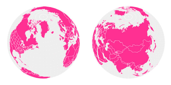
I hope you enjoyed this tutorial! Have fun with your vector globes!